BST / AVL Tree Visualizer

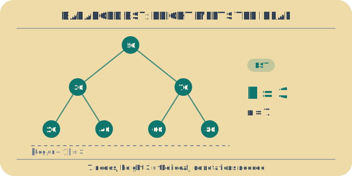
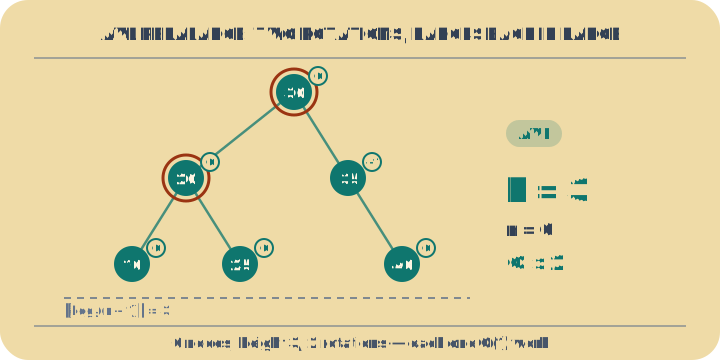
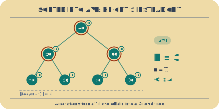
Binary Search Trees mandate a strict hierarchical organization, ensuring left-child nodes hold lesser values. AVL trees enhance this by algorithmically enforcing a maximum height differential of one between subtrees. This mathematical self-balancing requires precise rotational transformations upon insertion or deletion. Such structural constraints guarantee search, insertion, and deletion operations remain bounded by O(log n) time complexity, optimizing rapid data retrieval.

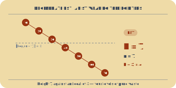
A binary search tree works like looking up a word in a dictionary: at each node you compare, then discard the entire half that cannot contain your value. That is why a well-shaped tree finds anything among a million entries in about 20 comparisons. But the shape depends entirely on insertion order — type the values already sorted (10, 20, 30, …) and watch the tree collapse into a single leaning line, no faster than scanning a list one by one.

Switch to AVL mode and ask: how tall can a balanced tree get for a given number of nodes? The answer hides the golden ratio. The sparsest legal AVL tree of each height is a Fibonacci tree, built from two smaller Fibonacci trees, so its node counts follow the Fibonacci sequence. That is why the height bound carries the constant 1.44 — it is exactly 1 / log₂(φ), with φ ≈ 1.618, the golden ratio.