BST / AVL Tree Visualizer

Insert values and watch the tree grow. Switch to AVL mode to see automatic rebalancing.

Loading interactive simulation...

Sorted input is the worst input 🖖

A binary search tree earns its speed from its shape, and the shape comes entirely from insertion order. Feed this tool 10, 20, 30, 40, 50, 60, 70 in that order and every key is larger than the last, so every one hangs off the right of the one before: the tree becomes a straight chain of height 7. It is a linked list carrying the overhead of tree pointers, and finding 70 costs seven comparisons instead of three. Nothing about the data was pathological — it was merely already sorted, which is how data usually arrives. Switch the same seven values to AVL mode and rotations force the height back to 3. That is the entire argument for self-balancing trees.

Every step throws away half 🖖

A binary search tree works like looking up a word in a dictionary: at each node you compare, then discard the entire half that cannot contain your value. That is why a well-shaped tree finds anything among a million entries in about 20 comparisons. But the shape depends entirely on insertion order — type the values already sorted (10, 20, 30, …) and watch the tree collapse into a single leaning line, no faster than scanning a list one by one.

The golden ratio hides in AVL trees 🖖

Switch to AVL mode and ask: how tall can a balanced tree get for a given number of nodes? The answer hides the golden ratio. The sparsest legal AVL tree of each height is a Fibonacci tree, built from two smaller Fibonacci trees, so its node counts follow the Fibonacci sequence. That is why the height bound carries the constant 1.44 — it is exactly 1 / log₂(φ), with φ ≈ 1.618, the golden ratio.

BST AND AVL TREES — THE SAME VALUES, FOUR DIFFERENT TREES

Which Tree Will Your Insert Order Give You?

A binary search tree's shape is not decided by which values it holds. It is decided by the order they arrived in, and that shape is the whole cost of using it: every search, insert and delete walks from the root to a leaf, so the height is the price. Two questions settle which case you are in — did the values arrive already sorted, and is anything rotating them back into balance?

Balanced BST — the arrival order interleaved h = 3 = ⌈log₂(n + 1)⌉
Degenerate BST — sorted input, nothing rebalancing h = n = 7 ⇒ O(n)
AVL rebalance — the rotation is local and cheap |hL − hR| > 1 → ↻, h = 3
AVL on sorted input — the case rotations exist for ↻ × 4 ⇒ h = 3 < 7

01

Balanced BST — the arrival order interleaved

What you know: Plain BST mode, no rotations. The values arrive middle-first, so each new key drops into a subtree that is still short and no side gets ahead of the other.

What it costs: h = 3 = ⌈log₂(n + 1)⌉

Worked example: 50, 30, 70, 20, 40, 60, 80 → root 50, 7 nodes, height 3 — exactly the ideal ⌈log₂(7+1)⌉ = 3, so the deepest search costs 3 comparisons

Open this case: Balanced
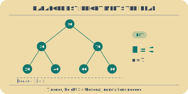
Balanced BST — the arrival order interleaved. Seven nodes on three levels: every leaf the same distance from the root, which is as good as it gets. Plain BST mode, no rotations. The values arrive middle-first, so each new key drops into a subtree that is still short and no side gets ahead of the other.
Seven nodes on three levels: every leaf the same distance from the root, which is as good as it gets.

02

Degenerate BST — sorted input, nothing rebalancing

What you know: Plain BST mode again, but the values arrive in ascending order. Each one is larger than everything already stored, so it goes right, every single time.

What it costs: h = n = 7 ⇒ O(n)

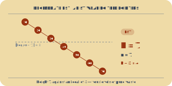
Worked example: 10, 20, 30, 40, 50, 60, 70 → root 10, 7 nodes, height 7 instead of 3; finding 70 takes 7 comparisons, and the tool labels the result a linked list

Open this case: Degenerate
Degenerate BST — sorted input, nothing rebalancing. Every node has one child: a search walks all seven levels, no faster than scanning an array. Plain BST mode again, but the values arrive in ascending order. Each one is larger than everything already stored, so it goes right, every single time.
Every node has one child: a search walks all seven levels, no faster than scanning an array.

03

AVL rebalance — the rotation is local and cheap

What you know: AVL mode. After each insert the tree walks back up towards the root, and the first node whose two subtree heights differ by more than 1 gets rotated. The badges next to each node show left height minus right height.

What it costs: |hL − hR| > 1 → ↻, h = 3

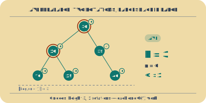
Worked example: 30, 20, 10, 25, 35, 40 in AVL mode → inserting 10 tips node 30 to +2, and one right rotation lifts 20 into its place; inserting 40 later tips a node to −2 and one left rotation fixes it. 2 rotations, 6 nodes, height 3.

Open this case: AVL rebalance
AVL rebalance — the rotation is local and cheap. The ringed nodes were lifted by a rotation; every badge is back within ±1. AVL mode. After each insert the tree walks back up towards the root, and the first node whose two subtree heights differ by more than 1 gets rotated. The badges next to each node show left height minus right height.
The ringed nodes were lifted by a rotation; every badge is back within ±1.

04

AVL on sorted input — the case rotations exist for

What you know: AVL mode, fed exactly the values that produced the chain two cases above. Every insert lands at the far right end and pushes an ancestor's balance to −2, so almost every insert triggers a fix.

What it costs: ↻ × 4 ⇒ h = 3 < 7

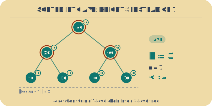
Worked example: 10, 20, 30, 40, 50, 60, 70 in AVL mode → 4 left rotations, and the root ends up as 40 rather than 10. Height 3, not 7 — the same input, the same seven nodes, less than half the depth.

Open this case: Sorted into AVL
AVL on sorted input — the case rotations exist for. The same sorted values as case 2, rotated back into three levels as they arrive. AVL mode, fed exactly the values that produced the chain two cases above. Every insert lands at the far right end and pushes an ancestor's balance to −2, so almost every insert triggers a fix.
The same sorted values as case 2, rotated back into three levels as they arrive.
References (1)
  • Insight block 3 — the Fibonacci tree that sets the AVL height bound: D. E. Knuth, The Art of Computer Programming, Volume 3: Sorting and Searching, 2nd edition, §6.2.3. Addison-Wesley, 1998. ISBN 978-0-201-89685-5 — the sparsest legal AVL tree of each height, and the logφ bound that follows.

Problem solved in full

  1. A tree of height seven with seven nodes 5 steps

    Seven nodes and a tree of height seven. A balanced tree would be height 3. Work out what the input did — and what that costs at scale.

    1. The default keys are 10, 20, 30, … — already sorted. Follow the insertion rule and every new key is larger than everything in the tree, so it goes right, every time.

    2. The result has no branching at all. Each node has one child, so the structure is a linked list that happens to be drawn as a tree, and the height equals the node count.

    3. The best possible height for seven nodes is 3, because a tree of height h holds at most 2ʰ − 1 nodes and 2³ − 1 = 7 exactly. This input achieves the worst case while the balanced case was available.

    4. Lookup walks from the root, so the cost is the height: 7 comparisons here against 3.

    5. The ratio is the point, and it grows. At a million nodes the balanced height is 20 and the sorted-input height is a million.

    Answer

    The tool prints a height of 7 for 7 nodes against an ideal of 3. The lesson is that O(log n) was never a property of the binary search tree — it is a property of the insertion order, and the most natural order a programmer will ever hand it, sorted data, is precisely the one that destroys it. That is the entire reason AVL and red-black trees exist: they cost a rotation or two per insert to make the guarantee unconditional. Switch the mode to AVL and watch the same seven keys settle at height 3.

Example problems