Hash Table Visualizer

Enter keys and watch how they map to slots. See what happens when collisions occur.

Loading interactive simulation...

The all-collide preset does not have a broken hash — it has the wrong table size 🖖

Its keys are 0, 8, 16, 24, 32 and 40, and the table holds 8 slots. Every one of those keys is a multiple of 8, so key mod 8 sends all six to slot 0 and the table degenerates into a single list. Nothing is wrong with the hash function: it is doing exactly what it promises. The fault is that the table size shares a factor with the pattern in the keys. That is the entire argument for prime table sizes — a size of 8 is helpless against keys that step by 8, while a prime size has no factor for the keys to land on. Switch to the probing presets and watch the same collision handled two different ways.

Jump straight to the slot 🖖

A hash table is just an array paired with a rule — the hash function — that turns any key into a slot number. Instead of scanning every entry one by one, you compute where an item belongs and go straight there, which is why lookups stay fast even with millions of keys. Speed depends on spreading keys evenly. Insert a few here and watch how quickly two keys want the same slot.

When collisions become a weapon 🖖

Because a hash table degrades to a slow linear scan when too many keys pile into one slot — exactly the worst case you can trigger above — an attacker who knows your hash function can craft thousands of keys that deliberately collide. In 2011 this 'hash-flooding' trick froze web servers in PHP, Java, Python, and Ruby with a single crafted request. The fix was randomly seeded hash functions like SipHash, now standard in many languages.

HASH TABLES — WHERE A KEY LANDS, AND WHAT HAPPENS WHEN TWO LAND TOGETHER

Which Collision Case Are You Handling?

A hash table is O(1) only while the keys spread out. Two questions settle everything: does the hash function scatter your keys, and when two of them do collide, do you hang the second one off the slot or go hunting for another slot? The load factor α = n/m decides how often collisions happen; the strategy decides what each one costs.

No collisions — the case the O(1) promise assumes h(k) = k mod m, α = n/m
Every key in one bucket — chaining degenerates to a list O(n)
Linear probing — open addressing with primary clustering (h + i) mod m
Quadratic probing — no clustering, but it can refuse to insert (h + i2) mod m

01

No collisions — the case the O(1) promise assumes

What you know: Every key hashes to a different slot. The load factor α = n/m is below 1 and the hash spreads the keys evenly across the table.

Probe rule: h(k) = k mod m, α = n/m

Worked example: keys 0–5 into m = 8 with h(k) = k mod 8 → slots 0–5, one probe each: α = 0.75 and an average of exactly 1.00 probes

Open this case: No collision
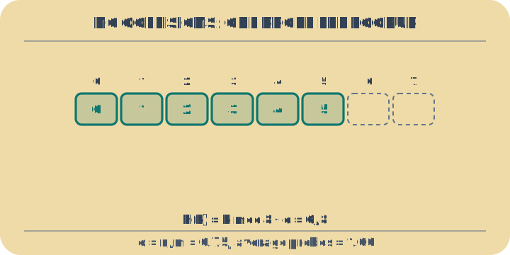
No collisions — the case the O(1) promise assumes. Six keys, six different slots, one probe each — the load factor is the only thing to watch. Every key hashes to a different slot. The load factor α = n/m is below 1 and the hash spreads the keys evenly across the table.
Six keys, six different slots, one probe each — the load factor is the only thing to watch.

02

Every key in one bucket — chaining degenerates to a list

What you know: All the keys are multiples of the table size, so k mod m gives the same slot for every one of them. Chaining still stores them all, but in a single chain.

Probe rule: O(n)

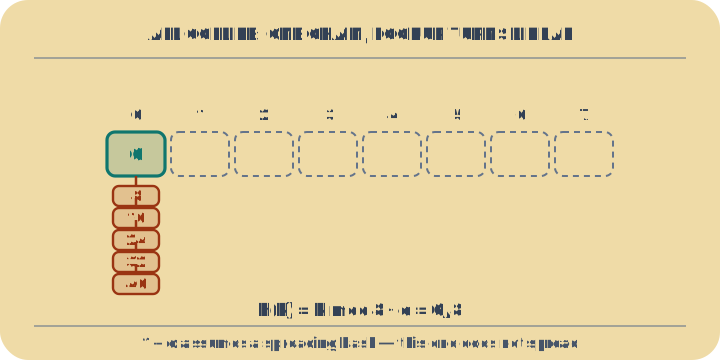
Worked example: keys 0, 8, 16, 24, 32, 40 into m = 8 → all land in slot 0; inserting them costs 1+2+3+4+5+6 = 21 probes, an average of 3.50

Open this case: All collide
Every key in one bucket — chaining degenerates to a list. All six keys in slot 0: a hash table that has quietly become a linked list. All the keys are multiples of the table size, so k mod m gives the same slot for every one of them. Chaining still stores them all, but in a single chain.
All six keys in slot 0: a hash table that has quietly become a linked list.

03

Linear probing — open addressing with primary clustering

What you know: No chains: on a collision, step forward one slot at a time until an empty one appears. Every entry lives in the table itself.

Probe rule: (h + i) mod m

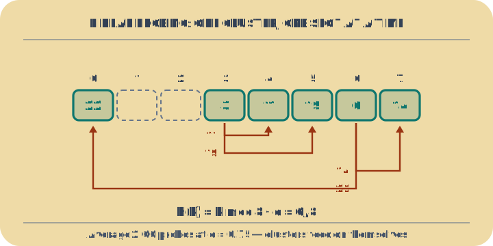
Worked example: keys 3, 11, 19, 6, 14, 22 into m = 8 → slots 3, 4, 5, 6, 7, 0 taking 1, 2, 3, 1, 2, 3 probes: average 2.00, and the six entries form one unbroken run

Open this case: Linear probing
Linear probing — open addressing with primary clustering. Occupied slots merge into one run; a key hashing inside it must walk all the way to the end. No chains: on a collision, step forward one slot at a time until an empty one appears. Every entry lives in the table itself.
Occupied slots merge into one run; a key hashing inside it must walk all the way to the end.

04

Quadratic probing — no clustering, but it can refuse to insert

What you know: On a collision, jump i² slots instead of i. That breaks up the clusters, but the probe sequence no longer visits every slot.

Probe rule: (h + i2) mod m

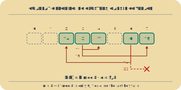
Worked example: the same keys into m = 8 → 3, 4, 7, 6, 2 — and then 22 fails outright: with m a power of two, i² mod 8 only ever equals 0, 1 or 4, so three slots are all it can reach

Open this case: Quadratic probing
Quadratic probing — no clustering, but it can refuse to insert. The probe sequence jumps and then repeats: empty slots remain and the last key has nowhere to go. On a collision, jump i² slots instead of i. That breaks up the clusters, but the probe sequence no longer visits every slot.
The probe sequence jumps and then repeats: empty slots remain and the last key has nowhere to go.

Problems solved in full

  1. A 75% full table averaging 3.5 probes per lookup 5 steps

    The table is 75% full and averages 3.5 probes per lookup. The standard formula for linear probing predicts 2.5 at that load. Find out which of the two is wrong.

    1. Neither is wrong, and the reason is in the keys. Hash each of the six with the table's own function and every one of them returns 3 — they are an arithmetic progression with common difference 8, and the table has exactly 8 slots.

    2. The load factor is still an honest 0.75: six keys in eight slots. It simply says nothing about where they went.

    3. So the probe sequence is the worst one available. The first key lands free; the second walks one slot; the third walks two. Six keys cost 1 + 2 + … + 6 = 21 probes, of which 15 are the extra work the panel reports.

    4. That is 3.5 probes per lookup on average.

    5. The textbook estimate assumes keys scatter uniformly, and at α = 0.75 it gives 2.5. The gap between 2.5 and 3.5 is not error — it is the cost of a hash function that shares a factor with the table size, applied to keys that share it too.

    Answer

    The tool prints α = 0.75, 15 probes of extra work and an average of 3.5. The lesson is that the load factor is the famous number and the wrong one to watch alone: it is identical here to a table holding six well-scattered keys, which would cost 2.5. What changed is the interaction between the key set and the modulus. This is why table sizes are chosen prime, and why hashing a struct by a field that happens to be a multiple of the capacity turns O(1) into O(n) with every metric still looking healthy. Change the size from 8 to 7 and watch the average collapse.

  2. A real hash map resizing at load factor 0.75 6 steps

    The panel puts 6 keys in 8 slots, load factor 0.75, and reports 3.5 probes. A successful lookup at that load costs about 2.5 probes — comfortable. So why does every real hash map resize at exactly 0.75 rather than filling up?

    1. Start where the panel is. Three quarters full, which sounds like sensible use of the memory.

    2. The successful search is the reassuring number: on average you check about two and a half slots before finding the key you wanted.

    3. The unsuccessful search is a different formula, and the difference is the whole answer. A miss must walk to the end of a run of occupied slots to prove absence — so the gap term is squared, not linear.

    4. Push the load a little higher and read what the square does. From 0.75 to 0.90 is a modest-sounding change of occupancy.

    5. Compare the two growth rates over that same step. The hit cost slightly more than doubles; the miss cost grows by a factor of six.

    6. So the table doubles instead. Every key is rehashed, which costs m operations, but it buys m more insertions before it happens again.

    Answer

    A miss at 0.75 costs 8.5 probes; at 0.90 it costs 50.5, and at 0.95 it costs 200.5. That is why 0.75 is the resize threshold in one standard library after another — it is not a memory-versus-speed compromise so much as the last point before the cliff. And the number that matters is the miss, because a miss is what every insertion does first, and what every failed lookup does entirely. The reassuring 2.5 on a successful search describes the case you were not worried about.

Learning path

When two things land on the same value

References (1)
  • Hashing, collision resolution and why table size matters, at length: Donald E. Knuth, The Art of Computer Programming, Volume 3: Sorting and Searching, 2nd edition, §6.4. Addison-Wesley, 1998. ISBN 978-0-201-89685-5.

Example problems

  • No collision - Keys 0 to 5 in a table of 8: six different slots, one probe each, not a collision anywhere. The load factor is already 0.75.
  • All collide - Every key is a multiple of 8, so all six hash to slot 0 and the chain runs six deep. That averages 3.5 probes - the figure the worked problem starts from.
  • Linear probing - 3, 11 and 19 all want slot 3; 6, 14 and 22 all want slot 6. Linear probing places all six, at 1, 2, 3, 1, 2, 3 probes, averaging 2.
  • Quadratic probing - The same six keys, and quadratic probing cannot place the last one. Squares mod 8 are only 0, 1 and 4, so from slot 6 the sequence reaches 6, 7 and 2 and nothing else - while slots 0, 1 and 5 stay empty.