Numerical Integration Lab

Estimate area under a curve or between two functions, and visualize how numerical methods approximate the integral.

Loading interactive simulation...

why Simpson can feel almost exact 🖖

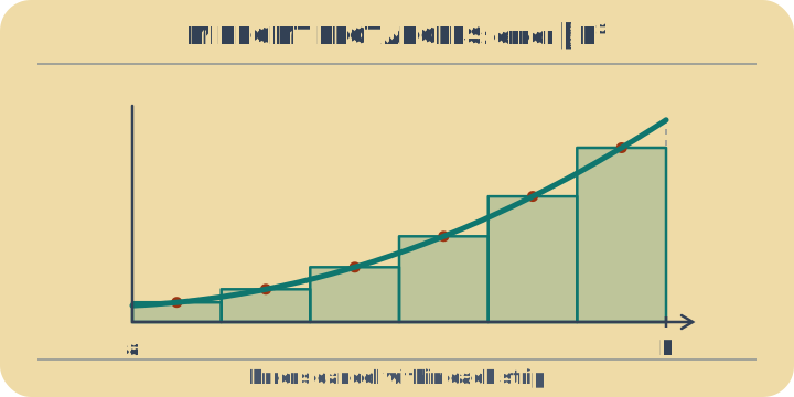
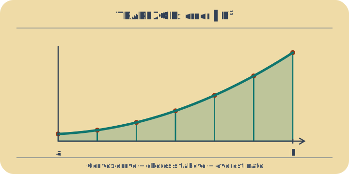
Numerical integration is not only about getting one estimate, it is about understanding error behavior. Left and right sums carry endpoint bias, midpoint and trapezoid usually improve with second-order convergence on smooth functions, and Simpson often improves much faster. When doubling n barely changes the estimate, your approximation is likely in a stable regime.

zoom in and every curve goes straight 🖖

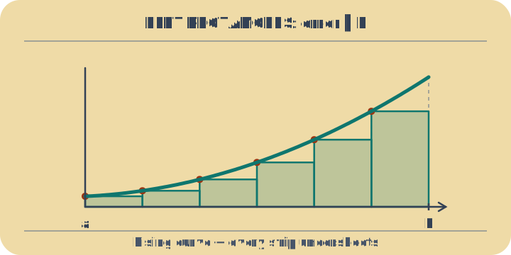
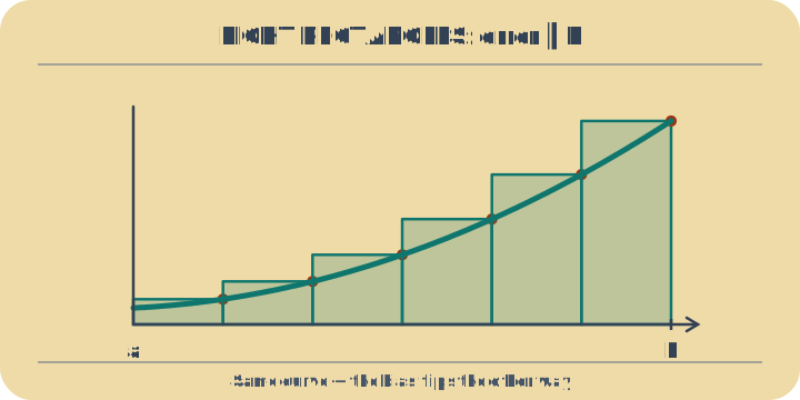
Numerical integration works by chopping the region under a curve into thin slices and filling each one with a simple shape — a rectangle, a trapezoid, or a little parabola — then adding the pieces up. The trick is that inside one narrow strip even a wild curve looks almost straight, so a crude shape fits surprisingly well. Watch the cyan fill: the thinner you make the slices, the less your choice of shape matters, because there is less curve left to miss.

Simpson's rule is older than Simpson 🖖

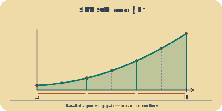
The panel formula this tool uses for Simpson, S = (Δx/6)(f(x_L) + 4f(x_M) + f(x_R)), is identical to a rule Johannes Kepler published in 1615 to gauge the volume of wine barrels — the Keplersche Fassregel — more than a century before Thomas Simpson wrote it down in 1743. It is a classic case of a method's name outliving its true inventor. Kepler needed it because a barrel's bulging side has no simple area formula.

Example problems

  • Coarse left - High n with left rectangles still shows left-endpoint bias on a convex curve.
  • Simpson smooth - On smooth sin(x), Simpson converges quickly to the true area.
  • Exp curved - For exp(x), trapezoid tends to overestimate because the curve is convex up.
  • Inverse tan - Midpoint captures the bounded 1/(1+x^2) profile with moderate partitions.
  • Between parabola and line - Difference integration tracks signed area between parabola and line.
  • Between sin and cos - Between-curves mode integrates sin(x)-cos(x) over the selected interval.
  • Custom - Custom presets combine transformed parabola and line coefficients in one scenario.