Hardy-Weinberg Equilibrium

Three views: watch allele frequencies evolve under genotype fitness, run a χ² test on observed genotype counts, and turn a disease incidence into carrier frequency.

Loading interactive simulation...

A real population could not hold that line 🖖

This tool never rolls dice. Its no-selection preset holds p = 0.500 for all fifty generations exactly, and running it a second time draws the identical curve, because there is no randomness anywhere in the model. No real population can behave that way. In a population of finite size, chance alone decides which individuals happen to breed, and that sampling error — genetic drift — nudges p every generation until one allele is eventually lost, with no selection involved at all. Drift bites harder the smaller the population, which is why conservation programmes worry about headcount even where nothing is selecting against the animals. Of the assumptions students skim past, infinite population size is the one doing the most work here.

Genotypes are just two random draws 🖖

At its heart, Hardy-Weinberg is simple probability. If alleles pair up at random, the chance of an AA child is just p × p = p², exactly like flipping two heads. That lets you work backwards: from the fraction of people affected by a recessive condition (q²) you recover how common the silent carriers are. If 1 in 10,000 is affected, then q = 0.01 and carriers (2pq) are about 1 in 50 — 200 times more common than the disease itself.

A pure mathematician's afterthought 🖖

This cornerstone of genetics came from someone who thought little of it. In 1908 the geneticist Reginald Punnett — a cricketing friend of G. H. Hardy at Cambridge — could not explain why a dominant trait didn't slowly take over a population. Hardy scribbled the answer, then published it almost apologetically, being a pure mathematician who disdained applied maths. The physician Wilhelm Weinberg derived the same law that year in German; it was ignored for 35 years until Curt Stern gave both men equal credit in 1943.

HARDY-WEINBERG — WHICH FORCE IS ACTING ON YOUR POPULATION?

Which Hardy-Weinberg Case Are You In?

Hardy-Weinberg is a null model: it says what a population does when nothing is acting on it. So the useful question is never whether the equation is true, but which of its assumptions your population breaks — because that is what decides which of the tool's three views you want. These six cases cover the baseline, the test that detects a departure from it, the three selection regimes the tool can simulate, and the one calculation that runs the equation backwards, from a disease rate to the allele hiding behind it.

No selection — the baseline w = 1 ⇒ p² + 2pq + q² = 1
Observed counts — test the fit χ² = 36.0 > 3.841, df = 1
Selection against the recessive — slow to finish w(aa) = 0.8 ⇒ q → 0
Heterozygote advantage — a stable polymorphism w(Aa) > w(AA), w(aa) ⇒ p → 0.667
Heterozygote disadvantage — an unstable tipping point w(Aa) < w(AA), w(aa) ⇒ p → 0 / 1
Backwards from incidence — counting carriers q = √(q²) ⇒ 2pq = 0.039

01

No selection — the baseline

What you know: An allele frequency p, and no fitness difference between the three genotypes.

Outcome: w = 1 ⇒ p² + 2pq + q² = 1

Worked example: p = 0.500 with all three fitnesses at 1. Genotypes sit at AA = 0.250, Aa = 0.500, aa = 0.250, and after 50 generations the tool still reports p = 0.500. Nothing has moved.

Open this case: Equal (p=0.5)
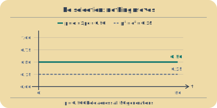
No selection — the baseline. All three fitnesses equal 1, so all five lines are flat. p and q never move, and the genotype frequencies stay at p², 2pq and q². An allele frequency p, and no fitness difference between the three genotypes.
All three fitnesses equal 1, so all five lines are flat. p and q never move, and the genotype frequencies stay at p², 2pq and q².

02

Observed counts — test the fit

What you know: Genotype counts from a real sample, and nothing else.

Outcome: χ² = 36.0 > 3.841, df = 1

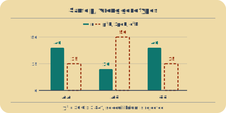
Worked example: AA = 40, Aa = 20, aa = 40 in a sample of N = 100. The tool estimates p̂ = 0.500, so it expects 25.00 / 50.00 / 25.00, and reports χ² = 36.000 against a critical value of 3.841 — p < 0.0001, so equilibrium is rejected.

Open this case: χ² test
Observed counts — test the fit. Observed counts against Hardy-Weinberg expectations. Both homozygotes are in excess while heterozygotes reach only 40% of expectation — a deficit worth χ² = 36.0 on one degree of freedom. Genotype counts from a real sample, and nothing else.
Observed counts against Hardy-Weinberg expectations. Both homozygotes are in excess while heterozygotes reach only 40% of expectation — a deficit worth χ² = 36.0 on one degree of freedom.

03

Selection against the recessive — slow to finish

What you know: The fitness of aa is below 1, while AA and Aa are equally fit.

Outcome: w(aa) = 0.8 ⇒ q → 0

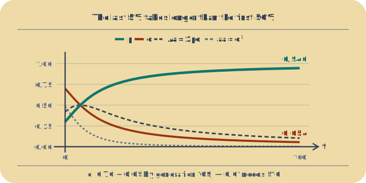
Worked example: p = 0.300 with w(aa) = 0.80. Over 100 generations the tool takes p to 0.946, so q falls from 0.700 to 0.054 — but not evenly. q is already past 0.500 by generation 7, reaches 0.050 at generation 109, and needs generation 516 to reach 0.010.

Open this case: Selection
Selection against the recessive — slow to finish. p climbs steeply and then stalls. The dashed aa line — the only genotype selection touches — collapses toward zero while the Aa line keeps the allele in circulation. The fitness of aa is below 1, while AA and Aa are equally fit.
p climbs steeply and then stalls. The dashed aa line — the only genotype selection touches — collapses toward zero while the Aa line keeps the allele in circulation.

04

Heterozygote advantage — a stable polymorphism

What you know: Aa is fitter than both homozygotes.

Outcome: w(Aa) > w(AA), w(aa) ⇒ p → 0.667

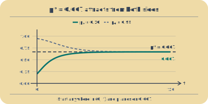
Worked example: p = 0.200 with w(AA) = 0.90, w(Aa) = 1.00, w(aa) = 0.80. The tool reports an internal equilibrium at p* = 0.667, and p climbs there from below — 0.657 by generation 50, 0.666 by generation 100.

Open this case: Overdominance
Heterozygote advantage — a stable polymorphism. p rises from 0.200 and flattens onto the dashed line at p* = 0.667. Both alleles persist indefinitely; neither is lost. Aa is fitter than both homozygotes.
p rises from 0.200 and flattens onto the dashed line at p* = 0.667. Both alleles persist indefinitely; neither is lost.

05

Heterozygote disadvantage — an unstable tipping point

What you know: Aa is less fit than both homozygotes.

Outcome: w(Aa) < w(AA), w(aa) ⇒ p → 0 / 1

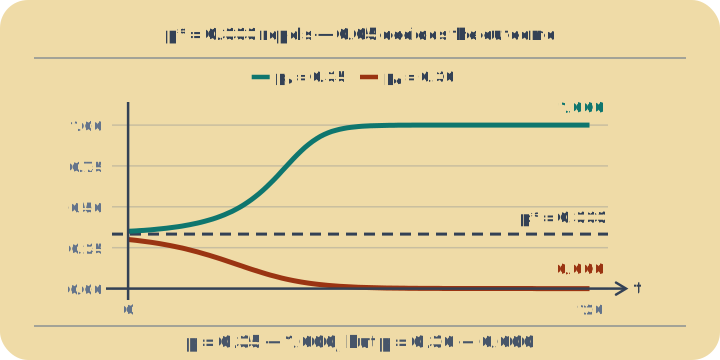
Worked example: p = 0.350 with w(AA) = 1.00, w(Aa) = 0.80, w(aa) = 0.90. The same p* formula gives 0.333, and the tool drives p to 1.000 by generation 80. Now set p to 0.300 — just below p* — and the identical three fitnesses take p to 0.000 instead.

Open this case: Underdominance
Heterozygote disadvantage — an unstable tipping point. Two runs with identical fitnesses. Starting just above p* = 0.333 fixes A; starting just below loses it. The dashed line is a watershed, not a destination. Aa is less fit than both homozygotes.
Two runs with identical fitnesses. Starting just above p* = 0.333 fixes A; starting just below loses it. The dashed line is a watershed, not a destination.

06

Backwards from incidence — counting carriers

What you know: How common the recessive condition is. Nothing about allele frequencies.

Outcome: q = √(q²) ⇒ 2pq = 0.039

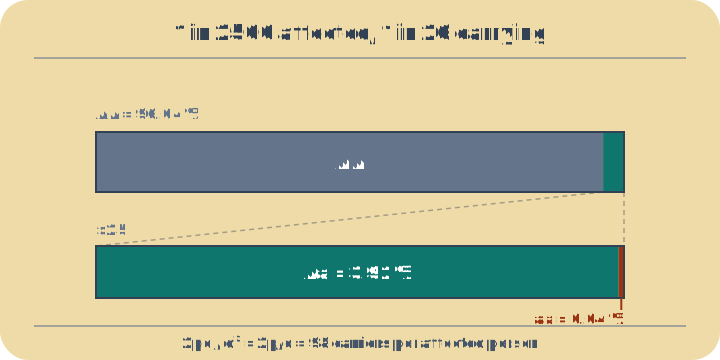
Worked example: An incidence of about 1 in 2500 births, so q² = 0.0004. The tool takes the square root to get q = 0.020, then p = 0.980, and reports carriers at 2pq = 0.039 — roughly 1 in 26 people.

Open this case: Cystic fibrosis
Backwards from incidence — counting carriers. The population bar at q = 0.020. The aa slice is 0.04% — too thin to label — while the Aa slice is 3.92%, ninety-eight times wider. How common the recessive condition is. Nothing about allele frequencies.
The population bar at q = 0.020. The aa slice is 0.04% — too thin to label — while the Aa slice is 3.92%, ninety-eight times wider.
References (5)

Problem solved in full

  1. Genotype proportions for a gene with two alleles at equal frequency 5 steps

    For a gene with two alleles at equal frequency, find the genotype proportions — then use the same identity to explain why a rare recessive disease cannot be bred out.

    1. If mating is random, an individual is two independent draws from the allele pool. The genotype frequencies are therefore the terms of a squared binomial, and they must sum to one.

    2. At p = q = 0.5 the split is a quarter, a half, a quarter. The calculator above prints exactly these, and the important feature is that they are stable — next generation gives the same, with no force required to maintain it.

    3. Now make the recessive allele rare, as a disease allele is. The affected frequency is q², which falls quadratically, but the carrier frequency 2pq falls only linearly.

    4. Take the ratio. Almost every copy of a rare allele is sitting in a healthy carrier, invisible to selection.

    5. So selection against the affected removes a vanishing share of the alleles each generation, and the decline follows a slow reciprocal, not an exponential.

    Answer

    0.250 : 0.500 : 0.250. At q = 0.01, one person in 10 000 is affected while one in 50 is a carrier — 198 carriers for every affected individual. Even eliminating every affected person from reproduction moves q from 0.0100 to only 0.0091 over ten generations, roughly 250 years. This is the population-genetics argument against eugenic programmes, and it is arithmetic rather than ethics: the allele is hiding in heterozygotes where selection cannot see it.

Example problems

  • Equal (p=0.5) - No fitness differences (all w = 1) with p = 0.5. Allele and genotype frequencies stay put generation after generation — the Hardy-Weinberg baseline.
  • Selection - The recessive homozygote aa is less fit (w = 0.8). The recessive allele slowly declines, and the change decelerates as remaining copies hide in Aa heterozygotes.
  • Overdominance - Heterozygote advantage — Aa is the fittest genotype, so both alleles are preserved and p settles at a stable equilibrium (~0.67) instead of one allele being lost.
  • Underdominance - Heterozygote disadvantage — Aa is the least fit genotype, so p = 0.35 is pushed away from the unstable point p* = 1/3 until A fixes. Drop p to 0.30 and the same three fitnesses lose A instead.
  • χ² test - Observed counts (AA=40, Aa=20, aa=40) that don't fit Hardy-Weinberg proportions; the χ² test flags a significant departure from equilibrium.
  • Cystic fibrosis - Cystic-fibrosis-like incidence (~1 in 2500 affected). Recover the recessive allele frequency and the carrier frequency from q².