BFS vs DFS Visualizer
Watch how BFS and DFS explore the same graph differently. BFS goes wide, DFS goes deep.
Topological Traversal and Complexity Bounds 🖖
Graph traversal algorithms are strictly defined by their data structure dependencies: queues for Breadth-First Search (BFS) and stacks for Depth-First Search (DFS). BFS expands radially, mathematically guaranteeing the shortest unweighted path, whereas DFS probes maximal depth before recursive backtracking. The time complexity for both remains strictly bounded by O(V + E). These deterministic traversal protocols dictate the computational efficiency of network analysis.
Same map, two travel styles 🖖
Run both side by side and you notice something: they visit the exact same nodes and edges, just in a different order. BFS explores its whole current neighbourhood before venturing further, so it has to remember every node waiting on the frontier. DFS commits to one branch and only tracks the path it is on. The practical takeaway: reach for BFS when the answer is likely close by, and DFS when the graph is deep and you want to keep memory small.
Both algorithms were born in mazes 🖖
Long before computers, DFS existed as a maze-walking rule published by the French mathematician Charles Pierre Trémaux in the 1800s. BFS arrived much later: Edward F. Moore reinvented it in a 1959 paper literally titled The Shortest Path Through a Maze, and Konrad Zuse had already sketched it in 1945. Two cornerstone algorithms of computer science, both first devised simply to escape a labyrinth.
Example problems
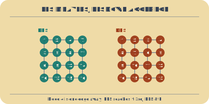
- 4x4 Grid - 4×4 grid: BFS explores layer-by-layer
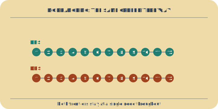
- Maze corridor - Maze corridor
- Star graph - Star graph
- Long chain - Long chain
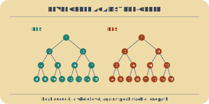
- Binary tree - Binary tree: DFS goes deep before wide
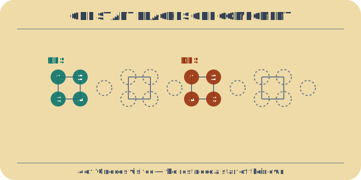
- Disconnected - Disconnected graph: unreachable nodes
- Dense graph - Dense graph: many edges, similar orders