Rational Functions Explorer

move zero/pole/gain and watch branch geometry change

Worked example — Rational Functions Explorer

\|z − p\|	3
x-intercept	1
Vertical asymptote	-2
Horizontal asymptote	1

These are the values the calculator shows when the page opens. Change any input above to recompute them.

Loading interactive simulation...

Put the zero on top of the pole and the blow-up vanishes 🖖

Drag the zero until it sits exactly on the pole and something odd happens: the curve stops exploding and flattens into a horizontal line. With z = p the factor (x − z) cancels the denominator outright, leaving the constant k everywhere — except at x = p, where the original formula still divides by zero. So the graph is a straight line with one point punched out of it, and this tool switches from reporting an asymptote to reporting a hole at (p, k). A denominator root is a pole only if the numerator does not cancel it; otherwise it is a removable hole, invisible at any zoom level.

Every curve here is a hyperbola 🖖

The tool computes f(x)=k(x−z)/(x−p): the distance from a zero divided by the distance from a pole, scaled by k. Whichever values you pick, the graph keeps the same shape — a hyperbola, the very curve that y=1/x draws. Sliding z and p only shifts it; changing k stretches it and flips which way the two branches open. Takeaway: master y=1/x and you have mastered them all.

A pole is only infinite by choice 🖖

Written as (ax+b)/(cx+d), any one-zero one-pole function is a Möbius transformation — the maps that rule complex analysis and hyperbolic geometry. Add a single point at infinity (the Riemann sphere) and the pole stops being a catastrophe: x=p simply maps to that new point, and x=∞ maps to the horizontal asymptote y=k. On the sphere the function is a smooth, reversible bijection — the "explosion" is just an artifact of the flat map.

RATIONAL FUNCTIONS — WHERE DOES THE GRAPH BLOW UP, AND WHERE DOES IT SETTLE?

Which Rational-Function Case Are You In?

f(x) = k(x − z)/(x − p) has only three numbers in it, and each one owns a feature of the graph. The zero z is where the curve crosses the axis. The pole p is where the denominator vanishes and the curve runs off to infinity. The gain k is where it settles far from both. Read those three off the formula and you have sketched the graph before plotting a single point.

Well separated — one vertical asymptote, one horizontal, one crossing x = p, y = k

Pole and zero close together — a violent spike between them |z − p| → 0 ⇒ |f| → ∞

Negative gain — the same skeleton with the branches swapped k < 0 ⇒ f → −f

Pole and zero almost on top of each other — nearly a hole (z − p)/(z − p) = 1, z ≠ p

Well separated — one vertical asymptote, one horizontal, one crossing

What you know: A pole and a zero at a comfortable distance. The vertical asymptote stands at x = p, the horizontal one at y = k, and the curve crosses the axis at x = z.

Feature: x = p, y = k

Worked example: f(x) = (x − 1)/(x + 2): asymptote at x = −2, crossing at x = 1, and f → 1 far out in both directions. At x = 0 the value is −0.5.

Open this case: basic

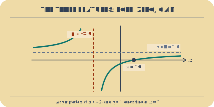
Well separated — one vertical asymptote, one horizontal, one crossing. The pole and the gain draw the two asymptotes; the zero fixes where the curve crosses. A pole and a zero at a comfortable distance. The vertical asymptote stands at x = p, the horizontal one at y = k, and the curve crosses the axis at x = z. — The pole and the gain draw the two asymptotes; the zero fixes where the curve crosses.

Pole and zero close together — a violent spike between them

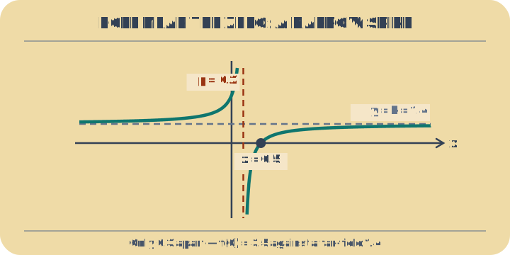
What you know: The same shape, but the pole sits near the zero. The curve has to get from the axis to infinity across a short distance, so it climbs steeply.

Feature: |z − p| → 0 ⇒ |f| → ∞

Worked example: f(x) = 1.4(x − 0.5)/(x − 0.2): the pole at 0.2 is only 0.3 from the zero at 0.5, and f(0) is already 3.5 against a far-field value of 1.4

Open this case: steep pole

$Pole and zero close together — a violent spike between them. A short gap between pole and zero forces the curve through a narrow, steep excursion. The same shape, but the pole sits near the zero. The curve has to get from the axis to infinity across a short distance, so it climbs steeply.$

A short gap between pole and zero forces the curve through a narrow, steep excursion.

Negative gain — the same skeleton with the branches swapped

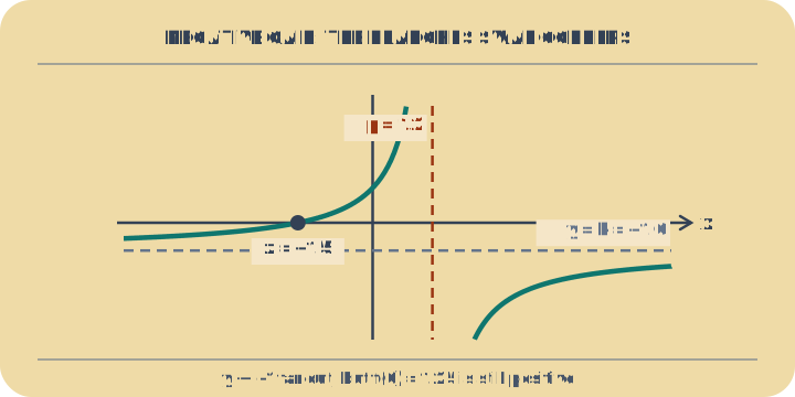
What you know: A negative k flips the whole curve about the horizontal axis. The asymptote positions do not move; the branches change which corner they occupy.

Feature: k < 0 ⇒ f → −f

Worked example: f(x) = −(x + 1.5)/(x − 1.2): asymptote at x = 1.2, crossing at x = −1.5, horizontal asymptote at y = −1, and f(0) = 1.25

Open this case: negative gain

Negative gain — the same skeleton with the branches swapped. The asymptotes are where they were, but each branch has moved to the opposite side. A negative k flips the whole curve about the horizontal axis. The asymptote positions do not move; the branches change which corner they occupy. — The asymptotes are where they were, but each branch has moved to the opposite side.

Pole and zero almost on top of each other — nearly a hole

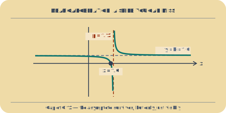
What you know: When z and p are very close, the factors almost divide out. Away from that neighbourhood the function is close to the constant k, and the pole survives as a needle-thin spike.

Feature: (z − p)/(z − p) = 1, z ≠ p

Worked example: f(x) = (x − 1)/(x − 1.12): only 0.12 apart, so f(0) = 0.893, close to the far-field value of 1 — yet the asymptote at x = 1.12 is still there

Open this case: near cancel

$Pole and zero almost on top of each other — nearly a hole. Almost a constant everywhere, except for the narrow window where the pole still wins. When z and p are very close, the factors almost divide out. Away from that neighbourhood the function is close to the constant k, and the pole survives as a needle-thin spike.$

Almost a constant everywhere, except for the narrow window where the pole still wins.

Common wrong intuition

A zero near a pole does not erase instability automatically. Near-cancellation can still be numerically sensitive.

Problem solved in full

The curve reaching its horizontal asymptote at y = 1 5 steps
f(x) = (x − 1)/(x + 2) has a horizontal asymptote at y = 1. Work out whether the curve ever actually reaches it.
1. The zero and the pole read straight off the factored form: the numerator vanishes at 1, the denominator at −2.
  
  $f (x) = 0 ⟺ x = 1; x + 2 = 0 ⟺ x = - 2 (vertical asymptote)$
2. For large |x| both top and bottom are dominated by their x terms, so the ratio tends to the ratio of leading coefficients. That is the horizontal asymptote, and here it is 1.
  
  $x \to \pm \infty lim \frac{x - 1}{x + 2} = \frac{1}{1} = 1 (horizontal asymptote)$
3. Now ask the question directly instead of eyeballing the graph: set the function equal to its asymptote and solve.
4. The x cancels and leaves −1 = 2, which is false for every x. So the curve never touches y = 1 — not far out, not anywhere.
  
  $\frac{x - 1}{x + 2} = 1 ⟺ x - 1 = x + 2 ⟺ - 1 = 2 — no solution$
5. The vertical asymptote behaves oppositely. Just left of −2 the function is −299; just right of it, +301. It does not approach a value from both sides, it diverges in opposite directions.
  
  $f (- 1.99) = - 299, f (- 2.01) = + 301$
Answer

The tool prints an x-intercept of 1, a vertical asymptote at −2 and a horizontal one at 1. The result worth keeping is that a horizontal asymptote is not a barrier — this one is never met, but that is a fact about this function and not a rule. Change the numerator to x − 1 + something that vanishes and a curve can cross its horizontal asymptote freely, even repeatedly. Vertical asymptotes are the strict ones: the function is undefined there, so it can never cross. Confusing the two is the most common mistake on this topic, and one line of algebra settles it every time.

$the curve approaches y = 1 and never reaches it; the pole flips sign$

Learning path

Beyond the quadratic

References (2)

Why k(x−z)/(x−p) is a Möbius map, and why circles and lines are the only shapes it produces: T. Needham, Visual Complex Analysis, Chapter 3: Möbius Transformations and Inversion. Oxford University Press, 1997.
The asymptotes as ordinary behaviour at a point, once infinity is a point: L. V. Ahlfors, Complex Analysis, 3rd edition. McGraw-Hill, 1979 — rational functions on the extended plane.

By the 42Math team · Updated 2026-07-27

Reviewed against published sources. Corrections welcome. Editorial policy · Corrections

All Mathematics lessons →

Example problems

basic - Basic one-zero one-pole shape with clear asymptotes.
steep pole - Pole near the origin creates strong local divergence.
negative gain - Negative gain flips branch orientation across asymptotes.
near cancel - Near-zero/pole cancellation mimics a removable-like behavior locally.