Riemann Sum Explorer

area approximation over partitions with method comparison

Worked example — Riemann Sum Explorer

Estimate	2.65625
True integral	2.66667
Absolute error	0.0104167
Signed error	-0.0104167
Lower sum	2.1875
Upper sum	3.1875
Upper-lower gap	1
Partition width	0.25

These are the values the calculator shows when the page opens. Change any input above to recompute them.

Loading interactive simulation...

why pharmacology switches rules halfway through 🖖

Drug exposure is a Riemann sum. A regulator wants the area under a patient's concentration-time curve; what exists is a dozen blood draws, so the standard method is the trapezoid rule between consecutive samples. That inherits the bias this page shows. An elimination curve is convex, the chord lies above it, and the linear trapezoid credits the patient with more exposure than they received. Hence the standard practice: linear up the absorption phase, logarithmic on the way down.

slicing area into shapes you can measure 🖖

Finding the exact area under a curve is hard, but adding up rectangles is easy. Each method here just guesses a strip's height differently: the left or right edge, the middle, or a slanted top (trapezoid). None is exact. But they close in at different speeds — double the strips and the left and right sums halve their error, while midpoint and trapezoid cut theirs by four.

Simpson's rule is a hidden blend 🖖

The midpoint rule usually beats the trapezoid rule, and their errors point in opposite directions — midpoint over-shoots where the curve is concave down, trapezoid under-shoots. Blend them as (2M + T)/3 and the leading error term cancels, giving Simpson's rule. So the most famous integration formula is just a weighted average of two sums already on this screen.

RIEMANN SUM THEORY — THE DEFINITION BEHIND THE INTEGRAL

Where Do You Sample Inside Each Strip?

A Riemann sum cuts [a, b] into n strips and gives each strip a single height, read off at one sample point inside it. Which point you tag — left edge, right edge, or middle — changes the answer while n is small. As n grows every choice closes on the same number, and that shared limit is what the definite integral means.

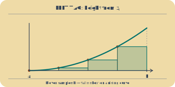
Left endpoint — tag at the start of each strip Σ f(x_i) Δx

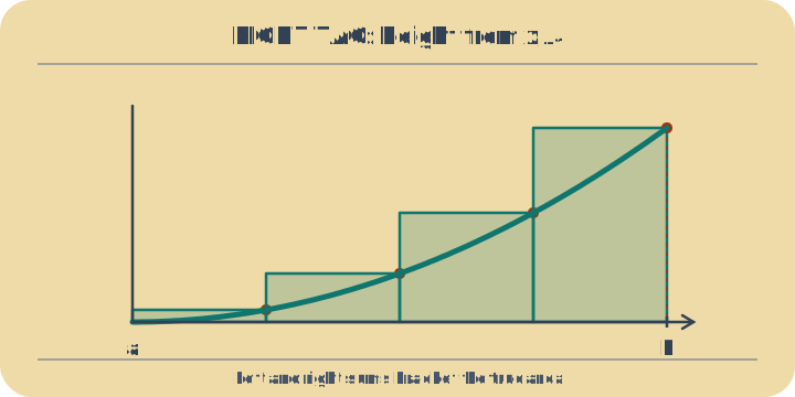
Right endpoint — tag at the end of each strip Σ f(x_i+1) Δx

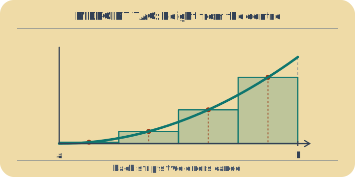
Midpoint — tag at the centre of each strip Σ f(x_i + Δx/2) Δx

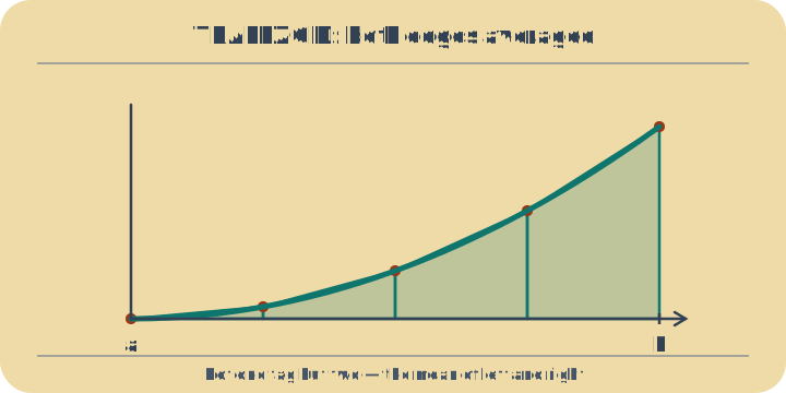
Trapezoid — both endpoints, averaged Σ ½[f(x_i) + f(x_i+1)] Δx

Left endpoint — tag at the start of each strip

Sample point: Height read at xᵢ, the left edge of strip i. The value at b is never used.

Sum: Σ f(x_i) Δx

At small n: x² on [0, 2] with n = 4 gives 1.75 against a true area of 2.667 — a long way short.

Open this case: coarse left

Left endpoint — tag at the start of each strip. Every rectangle takes its height from its own left edge, so a wedge of curve is left out. Height read at xᵢ, the left edge of strip i. The value at b is never used. — Every rectangle takes its height from its own left edge, so a wedge of curve is left out.

Right endpoint — tag at the end of each strip

Sample point: Height read at xᵢ₊₁, the right edge of strip i. The value at a is never used.

Sum: Σ f(x_i+1) Δx

At small n: Same curve and n: 3.75 against 2.667 — now overshooting by roughly what the left sum lost.

Open this case: right bias

Right endpoint — tag at the end of each strip. The same strips tagged at the right edge — now each rectangle overshoots. Height read at xᵢ₊₁, the right edge of strip i. The value at a is never used. — The same strips tagged at the right edge — now each rectangle overshoots.

Midpoint — tag at the centre of each strip

Sample point: Height read at the centre of the strip, so neither edge is privileged.

Sum: Σ f(x_i + Δx/2) Δx

At small n: Same curve and n: 2.625 against 2.667 — closer than left and right by an order of magnitude.

Open this case: refine n

Midpoint — tag at the centre of each strip. Sampling at the centre lets each strip’s two errors cancel against each other. Height read at the centre of the strip, so neither edge is privileged. — Sampling at the centre lets each strip’s two errors cancel against each other.

Trapezoid — both endpoints, averaged

Sample point: Both edges of the strip are used and the top is slanted between them.

Sum: Σ ½[f(x_i) + f(x_i+1)] Δx

At small n: Same curve and n: 2.75 against 2.667 — better than either endpoint sum, still behind midpoint.

Open this case: trapezoid smooth

Trapezoid — both endpoints, averaged. A slanted top joining both edges — the average of the left and right rectangles. Both edges of the strip are used and the top is slanted between them. — A slanted top joining both edges — the average of the left and right rectangles.

Problem solved in full

Estimating ∫₀² x² d x with eight midpoint rectangles 5 steps
Estimate ∫₀² x² dx with eight midpoint rectangles. Then do better than estimating: combine two wrong answers to get the exact one.
1. Eight strips across a width of 2 gives Δx = 0.25, and the midpoint rule takes each rectangle's height at the centre of its strip — 0.125, 0.375, and so on. Sampling at the centre is not an aesthetic preference; step 4 is what it buys.
  
  $Δ x = \frac{2 - 0}{8} = 0.25, x_{i}^{*} = 0.125, 0.375, \dots, 1.875$
2. Sum the eight squared midpoints and multiply by the common width. Nothing so far is approximate except the decision to use rectangles at all.
  
  $M_{8} = 0.25 i = 1 \sum 8 (x_{i}^{*})^{2} = 0.25 \times 10.625 = 2.65625$
3. The exact integral is 8/3, so the estimate is low by 0.0104167. Low, and by an amount worth explaining rather than shrugging at.
  
  $I = \int_{0}^{2} x^{2} d x = \frac{8}{3} = 2.66667 ⟹ M_{8} - I = - 0.0104167$
4. The midpoint error is −(b − a)h²f″(ξ)/24. For x² the second derivative is 2 everywhere, so it does not matter where ξ is, and the formula stops being a bound and becomes an equality. It returns −1/96, which is the tool's signed error to the last digit it prints.
  
  $E_{M} = - \frac{( b - a ) h ^{2}}{24} f^{''} (ξ) = - \frac{2 ( 0.25 ) ^{2} ( 2 )}{24} = - \frac{1}{96} = - 0.0104167$
5. The trapezoid rule errs the other way and by exactly twice as much: a midpoint rectangle cuts off as much as it adds, while a trapezoid chord lies wholly above a convex curve. Weight them two to one and the errors cancel.
  
  $T_{8} = 2.6875, T_{8} - I = + 0.0208333 = - 2 (M_{8} - I) ⟹ \frac{2 M _{8} + T _{8}}{3} = 2.66667$
Answer

Midpoint gives 2.65625 against a true 2.66667, bracketed by the lower and upper sums the tool prints at 2.1875 and 3.1875. But keep the last line: (2M + T)/3 = 8/3, exactly, from eight strips and no extra evaluations. That combination has a name — it is Simpson's rule, and this is where it comes from. It is not a cleverer way to draw rectangles; it is the observation that two crude methods fail in a fixed ratio, so their errors can be cancelled by construction. Switch the function to x³ and the tool prints a midpoint of 3.96875 and a trapezoid of 4.0625 — combine them and you get 4, dead on, because Simpson is exact for every cubic. Switch to x⁴ and it finally misses, by 6 parts in 100 000.

$M_{8} = 2.65625, E = - \frac{1}{96} \frac{2 M + T}{3} = \frac{8}{3} exactly$

Learning path

Why everything looks straight up close

Leads to Taylor series

References (4)

The definition itself, in the paper it first appeared in: B. Riemann, "Ueber die Darstellbarkeit einer Function durch eine trigonometrische Reihe." Abhandlungen der Königlichen Gesellschaft der Wissenschaften zu Göttingen 13, 87–132, 1867 — the section that asks what an integral is to mean for a function with infinitely many discontinuities, and answers with the sum this tool draws.
Upper and lower sums, and the criterion for the two to meet: G. Darboux, "Mémoire sur les fonctions discontinues." Annales scientifiques de l’École Normale Supérieure 4, 57–112, 1875.
How the definition was arrived at, and what it could not handle: D. M. Bressoud, A Radical Approach to Lebesgue’s Theory of Integration. Cambridge University Press, 2008.
Why medicine runs the trapezoid one way going up and another coming down: K. C. Yeh and K. C. Kwan, "A comparison of numerical integrating algorithms by trapezoidal, Lagrange, and spline approximation." Journal of Pharmacokinetics and Biopharmaceutics 6(1), 79-98, 1978.

By the 42Math team · Updated 2026-07-29

Reviewed against published sources. Corrections welcome. Editorial policy · Corrections

All Mathematics lessons →

Example problems

coarse left - Four left rectangles under x² give 1.75 against a true 2.666667. The (2M + T)/3 blend of those same four strips is exact.
refine n - Forty midpoint strips leave an error of 0.000417 where eight leave 0.010417. Five times the strips, twenty-five times the accuracy.
trapezoid smooth - sin(x) vanishes at both ends of [0, π], so left, right and trapezoid all return the identical 1.983524. Only midpoint, at 2.008248, differs.
concavity bias - e^x on [0, 1]: trapezoid reads 1.720519, midpoint 1.717164, truth 1.718282. The midpoint misses by half as much, the other way.
reverse interval - Integrating sin from π back to 0 returns -2.005723. Reversing the limits flips the sign and nothing else, because every strip width is now negative.
right bias - Six right rectangles overshoot to 3.370370 where six left ones give 2.037037. For a rising function the answer always sits between them.