Bayes Theorem / False Positive Explorer

how prevalence changes positive-test reliability

Loading interactive simulation...

why accuracy is only half the story 🖖

Sensitivity and specificity describe the test; prevalence describes the population before testing. Bayes theorem combines both. When prevalence is low, even a small false-positive rate can create many false alarms because most tested people do not have the condition. That is why a positive screening result often needs confirmation, while the same test can be highly persuasive in a high-risk group.

a test updates a belief, it doesn't replace it 🖖

Bayes theorem is a rule for changing your mind with evidence. You start with a prior โ€” your best estimate before testing, which here is the prevalence โ€” and the result nudges it up or down into a posterior. A single positive rarely jumps you straight to certainty; it multiplies your starting odds rather than overwriting them. The takeaway: before trusting any result, first ask how likely the thing was in the first place.

the same trap sent someone to prison 🖖

Confusing P(positive | disease) with P(disease | positive) has a courtroom name: the prosecutor's fallacy. In the 1999 trial of Sally Clark, a jury heard that two cot deaths in one family had a 1-in-73-million chance and treated it as the chance she was innocent. Those are different numbers โ€” the second ignores how rare the alternative (a double murder) also is. Her conviction was overturned in 2003, and the Royal Statistical Society publicly condemned the misuse.

BAYES โ€” A POSITIVE RESULT IS NOT THE SAME THING AS HAVING THE DISEASE

Which Screening Case Are You Reading?

Three numbers decide what a positive test means: how common the condition is, how often the test catches it, and how often it cries wolf. Sensitivity and specificity describe the test; prevalence describes the population โ€” and prevalence is usually the one doing the damage. Work in natural frequencies rather than percentages and the answer stops being counter-intuitive: imagine 1000 people, count the true positives, count the false ones, and compare.

Rare condition, excellent test โ€” most positives are still wrong PPV ≈ 9%
Common condition โ€” prevalence rescues a weaker test PPV ≈ 51%
Moderate prevalence โ€” and what a negative is worth PPV ≈ 60%, NPV ≈ 99%
High sensitivity, mediocre specificity โ€” the wrong dial PPV ≈ 29%

01

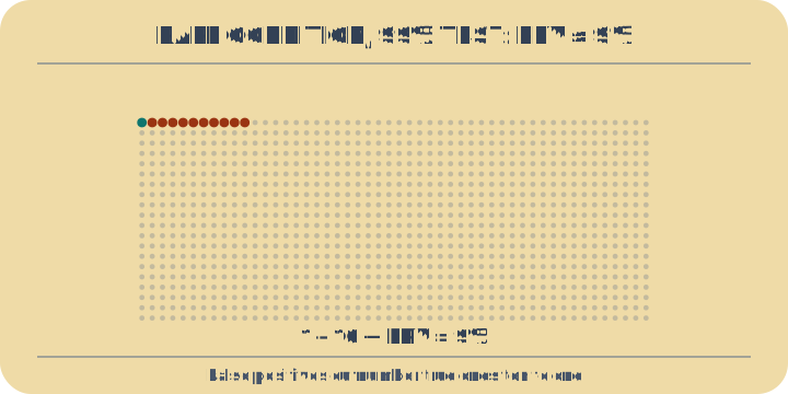
Rare condition, excellent test โ€” most positives are still wrong

What you know: Prevalence 0.1%, sensitivity 99%, specificity 99%. The test is as good as tests get; the condition is genuinely rare.

Result: PPV ≈ 9%

Worked example: Out of 10 000 people: 10 have it and about 10 test positive; 9990 do not and 100 of them test positive anyway โ†’ PPV = 10/110 โ‰ˆ 9%

Open this case: rare, accurate test
Rare condition, excellent test โ€” most positives are still wrong. Ten true positives are buried in a hundred false ones โ€” the base rate wins. Prevalence 0.1%, sensitivity 99%, specificity 99%. The test is as good as tests get; the condition is genuinely rare.
Ten true positives are buried in a hundred false ones โ€” the base rate wins.

02

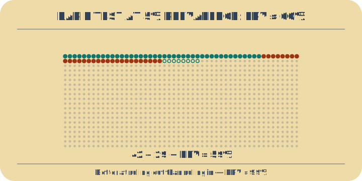
Common condition โ€” prevalence rescues a weaker test

What you know: Prevalence 10%, sensitivity 95%, specificity 90%. A distinctly worse test, applied where the condition is actually common.

Result: PPV ≈ 51%

Worked example: Out of 1000 people: 100 have it and 95 test positive; 900 do not and 90 test positive โ†’ PPV = 95/185 โ‰ˆ 51%

Open this case: more common disease
Common condition โ€” prevalence rescues a weaker test. Same arithmetic, ten times the prevalence: now a positive is roughly a coin flip. Prevalence 10%, sensitivity 95%, specificity 90%. A distinctly worse test, applied where the condition is actually common.
Same arithmetic, ten times the prevalence: now a positive is roughly a coin flip.

03

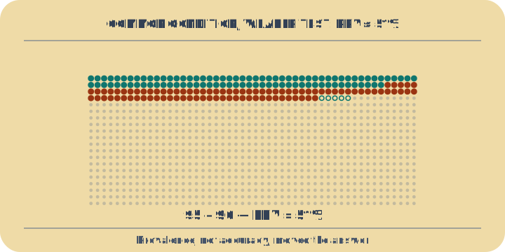
Moderate prevalence โ€” and what a negative is worth

What you know: Prevalence 5%, sensitivity 85%, specificity 97% โ€” the shape of a rapid antigen test during an outbreak.

Result: PPV ≈ 60%, NPV ≈ 99%

Worked example: Out of 1000: 50 infected, 43 caught and 7 missed; 950 clear, 29 wrongly flagged โ†’ PPV = 43/72 โ‰ˆ 60%, and NPV = 922/929 โ‰ˆ 99%

Open this case: covid-like
Moderate prevalence โ€” and what a negative is worth. A positive is a coin flip with a nudge; a negative is close to settled. Prevalence 5%, sensitivity 85%, specificity 97% โ€” the shape of a rapid antigen test during an outbreak.
A positive is a coin flip with a nudge; a negative is close to settled.

04

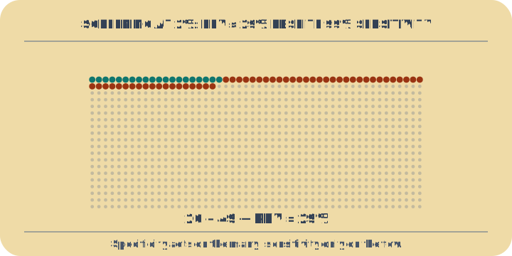
High sensitivity, mediocre specificity โ€” the wrong dial

What you know: Prevalence 2%, sensitivity 99%, specificity 95%. Almost nobody who uses is missed, but one healthy person in twenty is accused.

Result: PPV ≈ 29%

Worked example: Out of 1000: 20 users, 20 caught; 980 non-users, 49 flagged anyway โ†’ PPV = 20/69 โ‰ˆ 29%, so seven in ten positives are innocent

Open this case: drug screening
High sensitivity, mediocre specificity โ€” the wrong dial. Twenty real users against forty-nine false accusations: specificity is what needs fixing. Prevalence 2%, sensitivity 99%, specificity 95%. Almost nobody who uses is missed, but one healthy person in twenty is accused.
Twenty real users against forty-nine false accusations: specificity is what needs fixing.
References (1)

Problem solved in full

  1. A second positive result for a prevalence of 0.1% 5 steps

    A second positive result. This is prevalence 0.1% with sensitivity 99% and specificity 99% โ€” a rare condition and an excellent test, where one positive is famously weak evidence. Work out what a second, independent positive is worth.

    1. Odds, not probability, is the form in which evidence multiplies. One person in a thousand has the condition, so the starting position is 1 against 999 โ€” and it is that 999, not either dial, doing the damage.

    2. The likelihood ratio compares how often a positive turns up in each group. Both figures come off the dials: 99% of those with the condition test positive, and a specificity of 99% leaves 1% of everyone else testing positive as well.

    3. Multiplying prior odds by the likelihood ratio is the whole of Bayes in this form, and odds a against b convert back as a/(a+b). A factor of 99 is enormous evidence, and it still loses, because it started 999 behind.

    4. A second test begins where the first finished โ€” the posterior of one result is the prior of the next. Nothing about the test itself has changed, so the same factor of 99 applies, this time to odds that are no longer hopeless.

    5. That step assumed the two positives are independent, which is exactly what repeating the same test fails to give you. If whatever flagged a healthy person the first time โ€” a cross-reacting protein, a mislabelled sample โ€” flags them again half the time, the false positives barely thin out.

    Answer

    The tool prints 9.0% for a single positive, from a substitution that works out to 0.090164 โ€” the same 99/1098. Two independent positives make it 90.75% and three make it 99.90%, because the factor of 99 is charged every time while the 999-to-1 prior is paid for only once. That is the arithmetic behind confirmatory testing, and step 5 is its fine print: a correlated repeat lands on 16.4%, barely more convincing than the single result it was meant to confirm. The second test therefore has to fail differently from the first โ€” a different target molecule, a different laboratory, a different mechanism โ€” or the multiplication is fiction. The number to carry away is 99: sensitivity divided by false-positive rate is a test's entire evidential weight, and it is a multiplier on odds rather than an answer.

Learning path

Priors, and where they come from

Leads to Bayes' billiard the update with every input measurable.

Example problems

  • rare, accurate test - prev=0.1%, 99%-accurate test -> PPV only 9%: most positives are false alarms
  • more common disease - prev=10% -> PPV rises to 51%; prevalence is the hidden lever
  • covid-like - COVID rapid test at 5% prevalence -> PPV ~ 60%
  • drug screening - Drug screening at 2% prevalence -> PPV ~ 29% despite 99% sensitivity