Chi-Square and Residual Map
Change cell counts and watch significance and residual hotspots update immediately.
Goodness-of-fit boundaries and categorical variance 🖖
The chi-square test evaluates the association between categorical variables by comparing observed frequencies (O) with expected frequencies (E): χ² = Σ (O - E)² / E. Residuals show how much each individual category deviates from the null hypothesis expectation. The test assumes that expected cell counts are not too small (typically >= 5) to maintain the validity of the continuous approximation.
Where the association actually lives 🖖
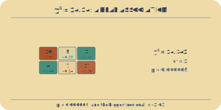
A single chi-square number and its p-value only tell you whether two categorical variables are linked at all — a yes-or-no verdict. The real story sits in the standardized residual map: each colored cell shows which specific combinations occur far more or far less often than independence would predict. A positive residual marks an over-represented pairing; a negative one marks an under-represented one. The practical takeaway: chase the brightest cells, not the largest raw counts.
Fisher's fix that Pearson refused 🖖
The degrees of freedom shown here, (r−1)(c−1), come from a bitter statistical feud. Karl Pearson introduced the chi-square test in 1900 but derived its degrees of freedom from the raw category count. In 1922 Ronald Fisher showed that every expected count estimated from the table's own margins costs one degree of freedom — which is why an r×c table has (r−1)(c−1), not rc−1. Pearson dismissed the correction for the rest of his life, yet Fisher was right, and it is the formula every table here uses.
Example problems
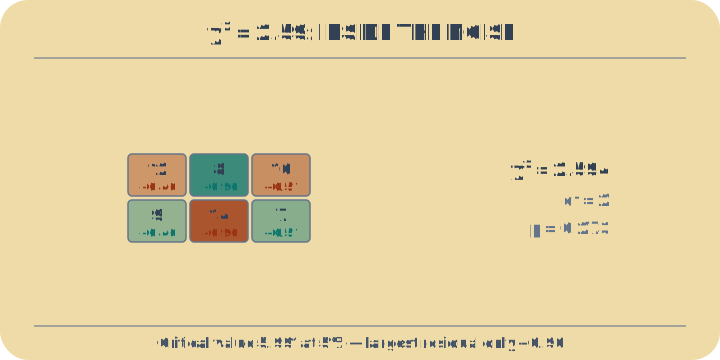
- Weak dependence - Weak dependence: moderate chi-square with small residual hotspots.
- Strong association - Strong association: large residual hotspots and high chi-square.
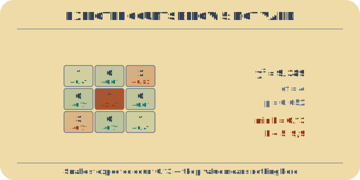
- Sparse warning case - Sparse table: expected-count warning highlights test limitations.
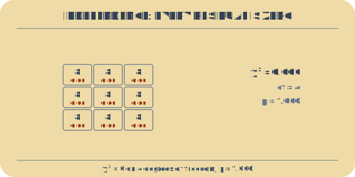
- Balanced baseline - Balanced table: near-independence with low residual magnitudes.