Student's t-Test

Perform hypothesis tests to determine if means differ significantly.

Worked example — Student's t-Test

t-statistic	4.1079
Degrees of freedom	29
p-value	0.0002982

These are the values the calculator shows when the page opens. Change any input above to recompute them.

Loading interactive simulation...

what p < 0.05 actually means 🖖

The p-value is the probability of observing a test statistic at least as extreme as yours, assuming H₀ is true. It is NOT the probability that H₀ is true. A p-value of 0.03 means: if the null were true, you'd see a result this extreme only 3% of the time by chance — unusual enough to reject. But 5% significance means 1-in-20 tests will reject a true null purely by accident (Type I error). Smaller α is stricter but increases Type II errors (missing real effects). The chart shows this directly: if the red line is past the amber threshold, p < α.

A signal-to-noise ratio for averages 🖖

At heart, the t-statistic is just a signal-to-noise ratio: the gap between your group means (the signal) divided by the standard error (the noise from random sampling). A big t means the difference stands out clearly from the scatter; a small t could easily be luck. The practical lesson: the same difference in means becomes more convincing as your samples grow or their spread shrinks, because that shrinks the noise in the denominator.

Welch's degrees of freedom aren't whole numbers 🖖

You might expect degrees of freedom to be a tidy integer — a count of independent pieces of information. But the Welch t-test uses the Welch–Satterthwaite formula, which typically returns a fractional value like df = 17.4. It is a deliberate approximation: when two groups have unequal variances, no exact whole-number df exists, so the method interpolates to match the true distribution as closely as possible. That is why Welch's df usually differs from the classic n₁ + n₂ − 2.

THE t-TEST — WHICH DESIGN, AND WHAT DOES THE VERDICT ACTUALLY SAY?

Which t-Test Case Are You In?

Two questions decide everything here. First the design: are you comparing one group against a claimed number, or two groups against each other? That fixes the formula and the degrees of freedom. Second the reading: a small p rejects the null, but a large one does not prove the null — it usually means the sample was too small to tell. Both mistakes are more common than arithmetic errors.

One sample against a claimed value — the evidence clears the bar t = (x̄ − μ₀) / (s/√n)

A smaller gap — no verdict, which is not the same as no effect p > α ⇏ H₀

Two independent groups — Welch, with no equal-variance assumption SE = √(s₁²/n₁ + s₂²/n₂)

The same comparison, underpowered — a difference the sample cannot resolve 1 − β ∝ δ√n/s

One sample against a claimed value — the evidence clears the bar

What you know: One group of measurements and a number to test it against. The statistic is t = (x̄ − μ₀)/(s/√n) on n − 1 degrees of freedom.

Statistic: t = (x̄ − μ₀) / (s/√n)

Worked example: x̄ = 78 against μ₀ = 72 with s = 8 and n = 30 → SE = 1.461, t = 4.108, df = 29, p = 0.0003

Open this case: Exam (reject H0)

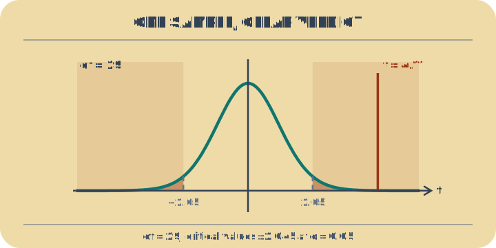
One sample against a claimed value — the evidence clears the bar. The observed t lands well outside the critical values, deep in the shaded rejection region. One group of measurements and a number to test it against. The statistic is t = (x̄ − μ₀)/(s/√n) on n − 1 degrees of freedom. — The observed t lands well outside the critical values, deep in the shaded rejection region.

A smaller gap — no verdict, which is not the same as no effect

What you know: Same design and the same n, but the difference is small next to the noise. p lands above α, so the null is not rejected.

Statistic: p > α ⇏ H₀

Worked example: x̄ = 73 against μ₀ = 72 with s = 8 and n = 30 → t = 0.685, p = 0.499

Open this case: Exam (fail to reject)

A smaller gap — no verdict, which is not the same as no effect. The observed t sits between the critical values, in the region where the test cannot decide either way. Same design and the same n, but the difference is small next to the noise. p lands above α, so the null is not rejected. — The observed t sits between the critical values, in the region where the test cannot decide either way.

Two independent groups — Welch, with no equal-variance assumption

What you know: Two separate samples, each with its own mean, spread and size. SE = √(s₁²/n₁ + s₂²/n₂), and the degrees of freedom come out fractional.

Statistic: SE = √(s₁²/n₁ + s₂²/n₂)

Worked example: 82 ± 10 from 40 subjects against 75 ± 12 from 38 → SE = 2.508, t = 2.791, df = 72.1, p = 0.0067

Open this case: Drug trial (sig.)

Two independent groups — Welch, with no equal-variance assumption. Two spreads, two sample sizes, and a df that is not a whole number — the signature of Welch. Two separate samples, each with its own mean, spread and size. SE = √(s₁²/n₁ + s₂²/n₂), and the degrees of freedom come out fractional. — Two spreads, two sample sizes, and a df that is not a whole number — the signature of Welch.

The same comparison, underpowered — a difference the sample cannot resolve

What you know: Two groups again, but smaller, with a smaller gap between them. The result is indistinguishable from noise.

Statistic: 1 − β ∝ δ√n/s

Worked example: 77 ± 11 from 25 subjects against 75 ± 12 from 28 → SE = 3.160, t = 0.633, df = 51.0, p = 0.530

Open this case: Drug trial (not sig.)

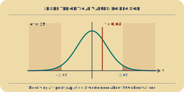
The same comparison, underpowered — a difference the sample cannot resolve. The observed t sits almost at the centre of the distribution, where nearly all of the probability lives. Two groups again, but smaller, with a smaller gap between them. The result is indistinguishable from noise. — The observed t sits almost at the centre of the distribution, where nearly all of the probability lives.

Problem solved in full

A sample of 30 scoring 78 where the population mean is 72 5 steps
A sample of 30 scores a mean of 78 where the claimed population mean is 72, with s = 8. Run the test — and then answer the question the p-value does not answer.
1. A single mean is a noisy estimate, and its noise is the standard error — the sample spread divided by the root of the sample size. Larger samples do not make individuals less variable; they make the average less variable.
  
  $SE = \frac{s}{n} = \frac{8}{30} = 1.4606$
2. The t-statistic asks how many standard errors separate what you saw from what was claimed. It is a distance measured in units of its own uncertainty.
  
  $t = \frac{x ˉ - μ _{0}}{SE} = \frac{78 - 72}{1.4606} = 4.1079$
3. Degrees of freedom are one fewer than the sample size, because the sample mean has already been spent estimating the centre. The calculator above prints both this and the statistic.
  
  $df = n - 1 = 29$
4. The p-value is the chance of a |t| this large if the claim were true. The tool prints 0.0002982 — about 3 in 10 000.
  
  $p = P (∣ T_{29} ∣ > 4.1079) = 0.0002982$
5. Now the part the p-value is silent about: how big the difference is. Cohen’s d divides by the spread of the data rather than the spread of the mean, and so does not shrink as the sample grows.
  
  $d = \frac{x ˉ - μ _{0}}{s} = \frac{6}{8} = 0.75$
Answer

t = 4.1079 on 29 df, p = 0.0002982. The effect size is d = 0.75, a genuinely large difference. Keeping the two apart is the whole discipline: p answers "could this be noise?", and it can be made arbitrarily small by collecting more data, because n appears in the standard error. d answers "does it matter?", and it does not move with n. A study with n = 10 000 can report p < 0.001 for a d of 0.02 — statistically certain, practically nothing.

$t = 4.1079, df = 29, p = 0.0002982 d = 0.75$

Learning path

When is a difference real?

Leads to ANOVA

References (1)

The paper that introduced the distribution, published under a pseudonym: "Student" (W. S. Gosset), "The Probable Error of a Mean." Biometrika 6, 1–25, 1908.

By the 42Math team · Updated 2026-07-27

Reviewed against published sources. Corrections welcome. Editorial policy · Corrections

All Statistics & Finance lessons →

Example problems

Exam (reject H0) - A class averaging 78 against a target of 72, spread 8, thirty students: t = 4.1079 and p = 0.0002982. The gap is six marks on a spread of eight, which is not a large effect, and it is decisive anyway — significance is set by the standard error of 1.4606, not by the size of the gap.
Exam (fail to reject) - Change the class average from 78 to 73 and nothing else: same spread, same thirty students. p goes from three in ten thousand to 0.499. Half of all classes drawn from a population that really does average 72 would sit at least this far from it. Failing to reject is not a finding that the difference is absent — it is the data declining to say.
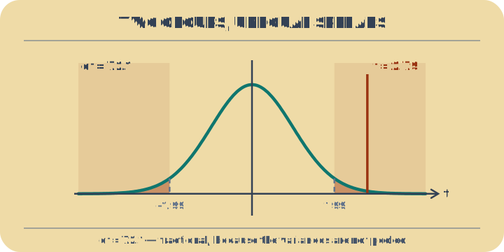
Drug trial (sig.) - Read the degrees of freedom: 72.137, not 76. Forty patients and thirty-eight would give 76 under Student's t, but the two spreads differ, 10 against 12, and Welch's correction charges for that in fractions of a degree. t = 2.7912 against a critical 1.9934, so p = 0.006716 and the result stands.
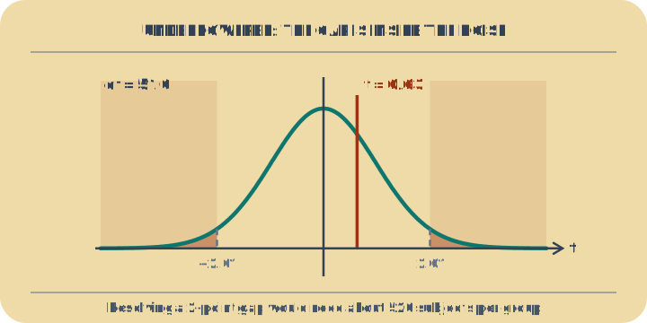
Drug trial (not sig.) - The same trial with a smaller gap and fewer patients: 2 points rather than 7, on 25 and 28 rather than 40 and 38. The standard error comes to 3.1596 — larger than the difference it is measuring — so t = 0.633 and p = 0.5296. Nothing here says the drug does not work. It says the trial was too small to find out.