Binomial Distribution Explorer

discrete success-count probabilities for fixed n and p

Starting values — Binomial Distribution Explorer

Trials (n)	20
Success probability (p)	0.35
Target successes (k)	7

Change any control above and the results recompute from these.

Loading interactive simulation...

Independence is the assumption that usually breaks first 🖖

The binomial needs three things to hold: a fixed number of trials, the same success probability p every time, and outcomes that do not influence one another. The first two are easy to check. The third quietly fails in most real situations.

Deal 5 cards from a deck and ask for the chance of 2 aces: the moment you draw one, p drops for every later draw, so the trials are not independent and the binomial is the wrong model — you need the hypergeometric. The rule of thumb is whether you are sampling with replacement or without. Put the card back and the binomial is exact; keep it and the binomial merely approximates, well when the deck is large relative to the hand and badly when it is not.

Counting successes in repeated trials 🖖

Imagine flipping the same biased coin n times and simply counting how many land heads. That count is a binomial random variable: each flip is independent, and every flip shares the same success probability p. The tool lets you slide n and p and watch where the probability piles up. Your best single guess for the number of successes is the mean, np — so 20 flips of a fair coin center on 10 heads.

Where the name really comes from 🖖

The "binomial" in binomial distribution is the same binomial as in algebra's binomial theorem. Expanding (p + q)ⁿ with q = 1 − p produces exactly the terms nCk · p^k · q^n−k — the probabilities for every k. Since (p + q) = 1, that expansion equals 1ⁿ = 1, which is why the probabilities must sum to one. The coefficients nCk are literally the rows of Pascal's triangle.

BINOMIAL PROBABILITY — WHICH QUESTION ARE YOU ACTUALLY ASKING?

Which Binomial Case Are You In?

The binomial needs three things and no more: a fixed number of independent trials n, the same success probability p in every one of them, and a count k. What changes from problem to problem is the question — exactly k, or at most k — and the shape that p gives the distribution. Decide those two and the arithmetic is mechanical.

Exactly k with p = ½ — the symmetric case P(X = k) = C(n,k) p^k(1−p)^n−k

At most k — sum the bars, do not read one P(X ≤ k) = ∑_i≤k P(X = i)

p far from ½ — the distribution leans μ = np, argmax P = ⌊(n+1)p⌋

Many trials, tiny p — the Poisson limit λ = np, P(X = k) ≈ e^−λλ^k/k!

Exactly k with p = ½ — the symmetric case

What you know: A fixed n, the same p in each trial, and a question about one specific count. With p = ½ the bars are symmetric about n/2.

Formula: P(X = k) = C(n,k) p^k(1−p)^n−k

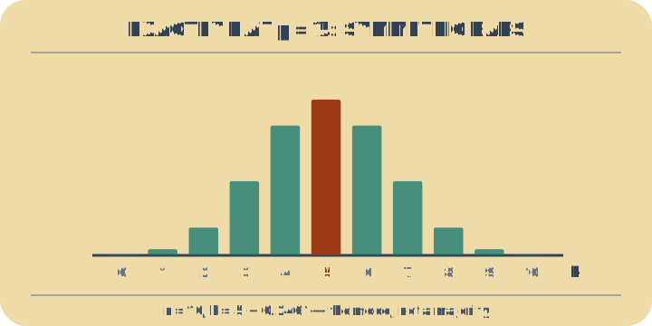
Worked example: n = 10, p = 0.5, k = 5 → C(10,5)·0.5¹⁰ = 252/1024 = 0.2461

Open this case: 10 fair coin flips

Exactly k with p = ½ — the symmetric case. With p = ½ the bars are symmetric about n/2, and even the tallest takes less than a quarter of the probability. A fixed n, the same p in each trial, and a question about one specific count. With p = ½ the bars are symmetric about n/2. — With p = ½ the bars are symmetric about n/2, and even the tallest takes less than a quarter of the probability.

At most k — sum the bars, do not read one

What you know: The question is a threshold rather than a single count. Add every bar from 0 up to k; one P(X = k) answers a different question entirely.

Formula: P(X ≤ k) = ∑_i≤k P(X = i)

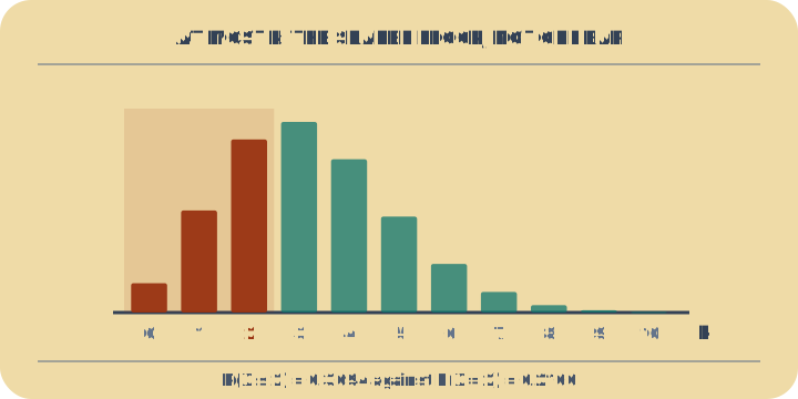
Worked example: n = 40, p = 0.08, k ≤ 2 → P(X ≤ 2) = 0.3694, while the single bar P(X = 2) is only 0.2100

Open this case: quality control defects

At most k — sum the bars, do not read one. The answer is the shaded block from 0 to k, not the height of the k-th bar. The question is a threshold rather than a single count. Add every bar from 0 up to k; one P(X = k) answers a different question entirely. — The answer is the shaded block from 0 to k, not the height of the k-th bar.

p far from ½ — the distribution leans

What you know: A lopsided success probability. The peak sits near np and the tail on the crowded side is squashed against the boundary at n.

Formula: μ = np, argmax P = ⌊(n+1)p⌋

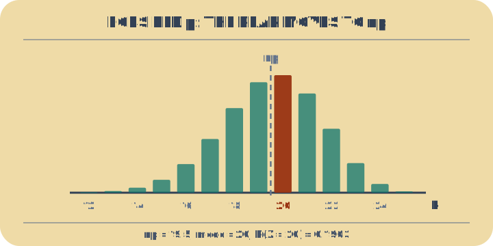
Worked example: n = 25, p = 0.78, k = 20 → 0.1903; the mean is np = 19.5 and the mode is ⌊(n+1)p⌋ = 20

Open this case: basketball free throws

p far from ½ — the distribution leans. A high p pushes the peak toward n and crushes the right tail against the boundary. A lopsided success probability. The peak sits near np and the tail on the crowded side is squashed against the boundary at n. — A high p pushes the peak toward n and crushes the right tail against the boundary.

Many trials, tiny p — the Poisson limit

What you know: n is large, p is small, and their product is a modest number. The binomial and a Poisson with λ = np agree to about two decimal places.

Formula: λ = np, P(X = k) ≈ e^−λλ^k/k!

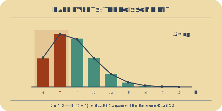
Worked example: n = 60, p = 0.03 → λ = 1.8; P(X ≤ 1) = 0.4592 exactly, against 0.4628 from the Poisson

Open this case: rare event process

Many trials, tiny p — the Poisson limit. The binomial bars and the Poisson with λ = np sit almost exactly on top of one another. n is large, p is small, and their product is a modest number. The binomial and a Poisson with λ = np agree to about two decimal places. — The binomial bars and the Poisson with λ = np sit almost exactly on top of one another.

Problems solved in full

Exactly 7 successes in 20 trials at p = 0.35 5 steps
Exactly 7 successes in 20 trials at p = 0.35. This is the PMF view with n = 20, p = 0.35 and k = 7. Build the bar from scratch, then work out its height a second time from the standard deviation alone.
1. The coefficient counts which 7 of the 20 trials are the successful ones, and nothing about the order they arrive in. Seven factors on top, 7! underneath — the cancellation is worth doing by hand once.
  
  $(7 20) = \frac{20 \times 19 \times 18 \times 17 \times 16 \times 15 \times 14}{7 !} = \frac{390 700 800}{5040} = 77520$
2. Every specific arrangement of 7 successes and 13 failures carries the same probability, because the trials are independent and p never moves. These are its two halves.
  
  $p^{k} = 0.3 5^{7} = 0.00064339, (1 - p)^{n - k} = 0.6 5^{13} = 0.00369721$
3. Multiply the number of arrangements by the probability of any one of them. The two probability factors together come to about 2.4 × 10⁻⁶, so it takes all 77,520 arrangements to lift the answer back up to 18%.
  
  $P (X = 7) = 77520 \times 0.00064339 \times 0.00369721 = 0.18440119$
4. The upper tail is not the complement of the cumulative figure: 1 − 0.6010266 would throw away k = 7, which belongs to both tails. The tool prints P(X ≤ 7) and P(X ≥ 7) but never P(X ≤ 6), so that subtraction is the reader's to do.
  
  $P (X \geq 7) = 1 - P (X \leq 6) = 1 - (0.6010266 - 0.1844012) = 1 - 0.4166254 = 0.5833746$
5. Now discard the factorials. A binomial whose mean sits well away from both 0 and n has the shape of a normal curve of the same standard deviation, and a normal curve's peak height depends on nothing else.
  
  $σ = n p (1 - p) = 4.55 = 2.133073, \frac{1}{σ 2 π} = \frac{1}{5.34682} = 0.18703$
Answer

The tool prints the coefficient 77,520, P(X = 7) = 0.18440119, P(X ≤ 7) = 0.6010266, P(X ≥ 7) = 0.58337458 and σ = 2.133073. Step 5 reaches 0.18703 from σ alone — 1.4% high, out of an expression containing neither n, nor p, nor a factorial. Raise n with p held at 0.35 and that error tracks 1/n: 0.71% at n = 40, 0.28% at n = 100, 0.07% at n = 400. So μ and σ are enough to sketch every bar near the middle, and the exact formula only earns its keep out in the tails — at k = 0 the same normal curve is 4.7 times too high, and at k = 17 it is 43% too low. Percentage errors in the middle, factor errors at the edges: that is the shape of every normal approximation you will meet.

$P (X = k) = (k n) p^{k} (1 - p)^{n - k} = 0.18440119 \approx \frac{1}{σ 2 π} = 0.18703$
60 trials at 3% where np is only 1.8 6 steps
This preset is 60 trials at 3%, and the panel gives P(X = 1) = 0.29840413. The normal approximation from the first problem is useless here — np is only 1.8. There is a different limit that is nearly exact, and it throws one of the two parameters away entirely.
1. The exact answer first, straight off the panel: sixty ways to place the single success, times the one success, times fifty-nine failures.
  
  $(1 60) (0.03)^{1} (0.97)^{59} = 60 \times 0.03 \times 0.16578007 = 0.29840413$
2. Hold the product np fixed and call it λ. That is the only quantity that is going to survive the limit.
  
  $λ = n p = 60 \times 0.03 = 1.8$
3. Take the combination term. Write p as λ/n, and the falling factorial divided by nᵏ tends to 1 as n grows — every factor is n minus something small, over n. What is left is λᵏ over k factorial.
  
  $(k n) p^{k} = \frac{n ( n - 1 ) \dots ( n - k + 1 )}{k !} (\frac{λ}{n})^{k} n \to \infty \frac{λ ^{k}}{k !}$
4. The failure term is the definition of e in disguise: (1 − λ/n) to the n tends to e^(−λ), and the extra k in the exponent stops mattering.
  
  $(1 - p)^{n - k} = (1 - \frac{λ}{n})^{n - k} n \to \infty e^{- λ}$
5. Put the two halves back together at k = 1.
  
  $P (X = 1) \approx λ e^{- λ} = 1.8 e^{- 1.8} = 0.29753800$
6. Now measure the error instead of asserting it is small.
  
  $\frac{0.29753800 - 0.29840413}{0.29840413} = - 0.0029$
Answer

0.29754 against the exact 0.29840 — 0.29% low, at only sixty trials. The Poisson limit keeps λ = np and forgets n and p separately, which is exactly why it describes situations where you never knew n at all: calls arriving at a switchboard, mutations per genome, typos per page. There is no trial count in any of those, only a rate. And the error falls like 1/n — at 600 trials of 0.3% it is 0.030%, at 6000 of 0.03% it is 0.003%. Ten times more trials, one tenth the error, with λ never moving.

$P (k) \to \frac{λ ^{k}}{k !} e^{- λ} : 0.29754 ⟷ 0.29840, - 0.29%$

Learning path

From counts to curves

Leads to Poisson the exact distribution of a count: n independent trials, each with the same probability p.

References (2)

Three centuries of the result this distribution was invented in order to prove: E. Seneta, "A Tricentenary history of the Law of Large Numbers." Bernoulli 19(4), 1088–1121, 2013 — on Jakob Bernoulli’s Ars Conjectandi of 1713.
And a shorter account of the book itself: I. Schneider, "Jakob Bernoulli, Ars conjectandi (1713)", in Landmark Writings in Western Mathematics 1640–1940, 88–104. Elsevier, 2005.

By the 42Math team · Updated 2026-08-17

Reviewed against published sources. Corrections welcome. Editorial policy · Corrections

All Statistics & Finance lessons →

Example problems

10 fair coin flips - Five heads in ten flips is the single most likely outcome, and it still happens under a quarter of the time: 0.2461. The most probable value of a binomial is usually not a probable value.
quality control defects - Forty units at an 8% defect rate averages 3.2 defects, so accepting a batch only when it has two or fewer rejects most batches that are behaving exactly as expected — the cumulative probability is 0.3694.
basketball free throws - A 78% shooter over 25 attempts averages 19.5 made. Landing on exactly 20 is the nearest whole number to that average and still only happens 19% of the time, which is how wide the distribution is at this n.
rare event process - Sixty trials at 3% averages 1.8 successes, so "at most one" is not the quiet outcome it sounds like: it happens 46% of the time, and getting none at all happens 16%.