Confidence Interval Calculator

mean/proportion intervals with live formulas

Starting values — Confidence Interval Calculator

Sample mean (x̄)	100
Sample standard deviation (s)	15
Sample proportion (p̂)	0.5
Sample size (n)	30

Change any control above and the results recompute from these.

Loading interactive simulation...

Overlapping error bars do not mean "no difference" 🖖

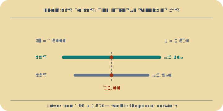
It is a standard move to draw two intervals, notice they overlap, and conclude the two things are not distinguishable. That test is far stricter than it looks. Two 95% intervals stop overlapping only once their estimates are 3.92 standard errors apart — and at that separation the difference between them carries a p-value of 0.0056. Actual significance at the 0.05 level arrives much earlier, at 2.77 standard errors. Between those two figures lies a band 1.15 standard errors wide, nearly a third of the way, in which the intervals plainly overlap and the difference is significant anyway. So insisting on a visible gap is roughly a p < 0.006 test: about nine times harsher than the 0.05 you thought you were applying, and a good way to miss a real effect.

A range beats a single guess 🖖

Any average or percentage you measure from a sample is almost never the exact truth, so this tool reports a range instead of one number. The margin of error is the "give or take" attached to your estimate. Here is the honest trade-off: from the very same data, a 99% interval is wider than a 90% one. More confidence buys less precision, so pick the level your decision actually needs.

The number behind "±3 points" 🖖

For a proportion the standard error is √(p(1−p)/n), and p(1−p) peaks at exactly p = 0.5 (value 0.25). Pollsters exploit this by assuming a 50/50 split as the worst case, which makes the 95% margin roughly 0.98/√n. Plug in n = 1000 and you get about ±3.1% — the classic poll figure. That is also why national polls rarely grow past ~1000 people: reaching ±1.5% would need four times the sample.

CONFIDENCE INTERVALS — WHAT ARE YOU ESTIMATING, AND HOW SURE DO YOU NEED TO BE?

Which Confidence-Interval Case Are You In?

Every interval has the same shape: the estimate, plus and minus a margin. What changes is where the margin comes from. Estimating a mean, the standard error is s/√n; estimating a proportion, it is √(p(1−p)/n). Then the confidence level picks the multiplier, and the sample size decides how much that multiplier costs you. Those three choices are the whole subject.

A mean at 95% — the default, and what the 95 actually refers to x̄ ± z·s/√n

Raising the confidence — a wider interval for the same data z: 1.96 → 2.576 (+31%)

A proportion — the standard error comes from p itself SE = √(p(1−p)/n)

A rare proportion — small p, and the approximation starts to strain np > 5, n(1 − p) > 5

A mean at 95% — the default, and what the 95 actually refers to

What you know: A sample mean with its standard deviation and size. The margin is z·s/√n, and at 95% the multiplier is 1.96.

Margin: x̄ ± z·s/√n

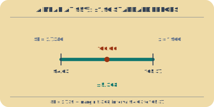
Worked example: x̄ = 100 with s = 15 and n = 30 → SE = 2.739, margin = 5.368, interval 94.63 to 105.37

Open this case: mean 95%

A mean at 95% — the default, and what the 95 actually refers to. The estimate sits at the centre, with 1.96 standard errors of margin on each side. A sample mean with its standard deviation and size. The margin is z·s/√n, and at 95% the multiplier is 1.96. — The estimate sits at the centre, with 1.96 standard errors of margin on each side.

Raising the confidence — a wider interval for the same data

What you know: The same kind of estimate at 99%. The multiplier rises from 1.96 to 2.576, so the interval widens by 31% even though nothing about the sample has changed.

Margin: z: 1.96 → 2.576 (+31%)

Worked example: x̄ = 72 with s = 12 and n = 64 → SE = 1.5, margin = 3.864, interval 68.14 to 75.86

Open this case: mean 99%

Raising the confidence — a wider interval for the same data. The same data at higher confidence: the centre is unmoved, the margin is longer. The same kind of estimate at 99%. The multiplier rises from 1.96 to 2.576, so the interval widens by 31% even though nothing about the sample has changed. — The same data at higher confidence: the centre is unmoved, the margin is longer.

A proportion — the standard error comes from p itself

What you know: Estimating a share rather than an average. There is no separate spread to measure: SE = √(p(1−p)/n), because for a yes-or-no outcome the variance is fixed by p.

Margin: SE = √(p(1−p)/n)

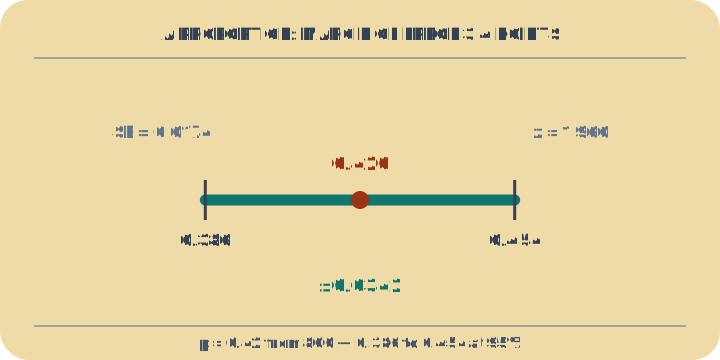
Worked example: p = 0.42 from n = 800 → SE = 0.0174, margin = 0.0342, interval 0.386 to 0.454 — a poll with a margin of error of 3.4 points

Open this case: proportion 95%

The interval is symmetric about the observed share, with a margin set by p and n alone.

A rare proportion — small p, and the approximation starts to strain

What you know: A small share estimated at high confidence. The interval is narrow in absolute terms but wide relative to p itself.

Margin: np > 5, n(1 − p) > 5

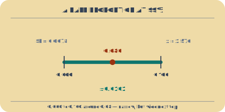
Worked example: p = 0.08 from n = 1200 at 99% → SE = 0.0078, margin = 0.0202, interval 0.060 to 0.100

Open this case: proportion 99%

A narrow interval in absolute terms, but a quarter of the estimate wide on each side.

Problem solved in full

The promise of a 95% confidence interval with n = 30 5 steps
What does the 95 in a 95% confidence interval actually promise? This is Mean CI with x̄ = 100, s = 15 and n = 30, at 95% confidence.
1. The interval is built around the sample mean, and the sample mean is itself random: repeat the study and it lands somewhere else. Its spread is the data's spread shrunk by √n, which is the only reason a larger sample buys precision.
  
  $SE = \frac{s}{n} = \frac{15}{30} = \frac{15}{5.4772} = 2.7386$
2. A two-sided 95% interval leaves 2.5% in each tail, so the multiplier is the standard normal value with 97.5% of the area below it. Because the 15 is a sample standard deviation from 30 observations, the stricter textbook choice is t₂₉ = 2.045; this panel uses z, the large-sample form, which moves each end of the interval by about a quarter of a unit.
  
  $z^{*} = Φ^{- 1} (\frac{1 + C}{2}) = Φ^{- 1} (0.9750) = 1.9600$
3. The multiplier converts standard errors into the units the measurement was made in, and the interval runs that far out on each side of the estimate.
  
  $ME = z^{*} SE = 1.9600 \times 2.7386 = 5.3677 ⟹ [94.6323, 105.3677]$
4. The 95% describes the recipe, not this interval: this one either contains the true mean or it does not, and nothing in the data tells you which. Repeat the whole study 100 times and each interval is an independent hit or miss with a 5% chance of missing, which makes the number of misses a binomial count rather than a fixed quota of five.
  
  $M \sim Bin (100, 0.05) : E [M] = 5, σ_{M} = 100 \times 0.05 \times 0.95 = 2.179$
5. A count that scatters by 2.179 is only surprising once it lands more than about two of those away from its own mean.
  
  $5 \pm 2 σ_{M} = [0.64, 9.36] M = 12 : z = \frac{12 - 5}{2.179} = 3.21$
Answer

A standard error of 2.7386 and a multiplier of 1.9600 give a margin of 5.3677, so the interval runs from 94.6323 to 105.3677. The part worth keeping is the last two lines: over 100 repeats of this study the misses average 5 but scatter with a standard deviation of 2.179, so anything from 1 to 9 misses is ordinary. Three misses is not evidence that the method is cautious and eight is not evidence that it is broken; you would need about 12, which is 3.21 standard deviations out, before the count says anything at all. The strip of green and red intervals is a picture of exactly that experiment, and its hit rate will not read 95 every time you look at it. A confidence level is a long-run property of the procedure, and 100 runs is not the long run.

$σ_{M} = N C (1 - C) = 2.179 misses on E [M] = 5$

Learning path

From counts to curves

References (1)

The paper that defined the confidence interval, and was careful about what the 95% is a statement about: J. Neyman, "Outline of a Theory of Statistical Estimation Based on the Classical Theory of Probability." Philosophical Transactions of the Royal Society A 236(767), 333–380, 1937.

By the 42Math team · Updated 2026-08-17

Reviewed against published sources. Corrections welcome. Editorial policy · Corrections

Example problems

mean 95% - Mean CI at 95% confidence for n=30, sd=15
mean 99% - Higher confidence widens interval even with larger n
proportion 95% - Proportion CI with moderate support and large sample
proportion 99% - Rare proportion estimate with high-confidence interval